Download
1 / 23
230 likes | 365 Vues
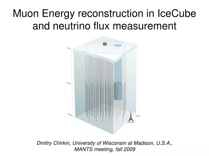
Muon Energy reconstruction in IceCube and neutrino flux measurement. Dmitry Chirkin, University of Wisconsin at Madison, U.S.A., MANTS meeting, fall 2009. Muon Energy reconstruction in IceCube. parameterization of light pattern created by a muon fitting of event data to this light pattern

E N D
Muon Energy reconstruction in IceCube and neutrino flux measurement Dmitry Chirkin, University of Wisconsin at Madison, U.S.A., MANTS meeting, fall 2009
Muon Energy reconstruction in IceCube • parameterization of light pattern created by a muon • fitting of event data to this light pattern • calibration of the fitted parameter to get the muon energy IceCube DOM 3 ATWD channels with gains ¼/2/16 Up to 12 ms combined waveform length Up to 200-300 p.e./10 ns charge resolution
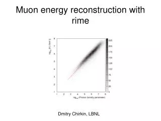
Number of photons vs. muon energy • In ice muon energy loss is dE/dx=a+bE with • a=0.26 GeV / mwe (1 mwe = 1/0.917 m of ice) • b=0.36 10-3 / mwe • A bare muon generates Cherenkov photons • This is about 32440 Cherenkov photons per meter of muon track at visible wavelengths. • From Geant-based simulations each cascade left by a muon generates as much light as a bare muon with the length of track of • 4.37 m E / GeV for electromagnetic cascades • 3.50 m E / GeV for hadronic cascades • For a typical muon the average is ~ 4.22 meters E/GeV • A typical cascade emits 4.22*32440 = 1.37 105 photons/GeV • for a muon track the “photon density parameter” is Area . Nc [m] = 32440 [m-1] (1.22+1.36 . 10-3 E/[GeV]) . 492.10 cm2. F = 2107.84 [m] (1.22+1.36 . 10-3 E/[GeV]) F=PMT efficiency, glass/gel transmission, etc.
Parameterization of the photon field left by a muon The flux function: total expected number of photons μ arriving at each OM. The parameterization of the flux function (as used by an icetray module MuE) is based on the following premises: μ = Nl · μ0(d), where Nl is the average number of photons emitted per unit length of a muon track and d is the distance to the track. precise if the muon track is infinite and emits the same number of Cherenkov photons per unit length anywhere along its track. In the immediate vicinity of the track: Far: We can stitch these together with
Other flux function parameterizations • based on PDF evaluated by explicit photon propagation simulations with photonics, which take into account the exact ice structure • semi-infinite muon parameterization • light saber (uniform cascades along track) • the above treatment employs layered ice treatment as well, but through the average scattering and absorption approximations. • fitting to decreasing amount of light along track • fitting to segments of the muon track • single OM energy estimates along track
Fitting data to the parameterized photon field likelihood function for the track hypothesis used in event reconstruction is: The total number of photons observed by an OM is: the corresponding expectation is: since In the presence of systematic uncertainties in the flux function, expression above can be integrated over the possibilities allowed by the uncertainties, or one employs the c2 sum minimization instead, with errors accounting for both statistical and systematic uncertainties.
Energy calibration with simulation and resolution Energy proxy: reconstructed number of cherenkov photons per unit length times effective area of the PMT ~ 0.3 Muon true (simulated) energy at the closest approach point to the center of gravity of hits in the event (weighted with charge)
dE/dx vs. number of Cherenkov photons • reconstructing dE/dx: a convenient approximation • number of Cherenkov photons is almost proportional to dE/dx • final “calibrated” energy parameter is what is most convenient to one’s analysis: • Rate of energy loss, or dE/dx: best, e.g., for muon bundles • Muon energy at closest approach point to center-of-gravity of hits
Muon energy reconstruction • Conclusions: • several light parameterization schemes exist • various fitting algorithms are used • Energy resolution of ~ 0.3 in log10(E [GeV]) is normally achieved
Neutrino energy spectrum unfolding • event selection • parameter distributions • smearing/unfolding matrix • summary of unfolding techniques • verifying the unfolding algorithm • measuring the neutrino spectrum
Event selection My own framework for applying cuts: SBM (subset browsing method) (simulated ns and ms) atmospheric ns atmospheric ms 2290 events 4492 events 8548 events 95% ~90% 99% purity 2290 events 4492 events 8548 events 90 – 180o 90 – 120o 120 – 150o 150 – 180o 30 parameters identified to separate signal and background Step 1: constructs surface separating signal from background Step 2: additional requirements for similarity with simulated signal 275.5 days of IceCube (22 strings) taken in 2007
Muon energy resolution reconstructed muon energy distribution simulation data True (from simulation) muon energy distribution Precision of the energy measurement: reconstructed vs. simulated true: ~ 0.3 in log10(E)
Parameter distributions Reconstructed zenith angle distribution vertical up horizontal Center of gravity (COG), or “average” event depth data simulation data simulation 2400 2200 2000 1800 1600 center of gravity depth [m] Point-spread function (PSF): Median angular resolution is ~ 2o.
Neutrino energy from reconstructed muon energy What we have: muon energy at detector with 0.3 in log10(E) resolution and its zenith angle with ~1.5o resolution What we want: muon neutrino energy distribution The transformation matrix is known from the simulation and relates muon and neutrino numbers: m=An Transformation/unfolding matrix
Unfolding methods • Performance of the following unfolding methods was studied: • Simple inversion and no-regularization c2 and likelihood minimization • SVD (singular value decomposition): • regularizing with the 2nd derivative of the unfolded statistical weight • regularizing with the 2nd derivative of the unfolded log(flux) • This is the selected method as it has the best behavior for: constant spectral index regularization term goes to 0 best identification of deviations from the given spectrum • also added the likelihood term describing fluctuations in the unfolding matrix • Bayesian iterative unfolding: • with and without smoothing of the unfolding matrix
Statistical uncertainties The following method is selected: Expand the regularization term in the vicinity of the minimum: constant term sum of first derivatives, creating a bias for counts in each bin sum of second derivatives, which tightens the minimum Introduce modified likelihood function by keeping the Poisson sum, and only the bias term from the regularization term (so that the minimum found during the unfolding does not change). However, do not include the sum of second derivatives of the regularization term. Vary the unfolded counts in each bin (independently) till modified likelihood function increases by ½.
Errors from belt construction, ½-likelihood estimate From 1000 simulations For a single representative simulation
Including fluctuations of the smearing matrix preliminary cf. AMANDA-II 2000-3: ~ 1.2 99 38 1.9 0.5 15 0.1 4.6 2.1 0.3 Unfolded data For a single representative simulation
Unfolded data at 2 different quality levels preliminary preliminary
Unfolded data with only events in the top or bottom preliminary preliminary
Conclusions and Outlook preliminary • Despite some residual problems in detector simulation, agreement with Barr. et al. (Bartol) muon neutrino flux is demonstrated • Improving the simulation is actively pursued, and the result with reduced systematic (and smearing matrix statistical) uncertainties is forthcoming