Download

1 / 29
1.32k likes | 2.66k Vues
Panel Data Analysis. From Workshop at NSO during 22-26 September 2008. Outline. What are panel data? Why use panel data? Handling panel data in stata Describing panel data Within and Between variation Unobservables Testing the FE and RE assumptions. What are panel data?.

E N D
Panel Data Analysis From Workshop at NSO during 22-26 September 2008
Outline • What are panel data? • Why use panel data? • Handling panel data in stata • Describing panel data • Within and Between variation • Unobservables • Testing the FE and RE assumptions
What are panel data? Panel data are a form of longitudinal data, involving regularly repeated observations on the same individuals. Individuals may be people, households, firms, area ,etc Repeat observations may be different time periods or units within clusters (e.g. workers within firms)
Why use panel data? • Repeated observations on individuals allow for possibility of isolating effects of unobserved differences between individuals • We can study dynamics • The ability to make causal inference is enhanced by temporal ordering • Some phenomena are inherently longitudinal (e.g. poverty persistence; unstable employment)
But don’t expect too much • Variation between people usually far exceeds variation over time for an individual • A panel with T waves doesn’t give T times the information of a cross-section • Variation over time may not exist for some important variables or may be inflated by measurement error
Some terminology A balanced panel has the same number of time observations (T) on each of the n individuals An unbalanced panel has different number of time observations (Ti) on each individual A compact panel covers only consecutive time periods for each individual- there are no “gaps” Attrition is the process of drop-out of individuals from the panel, leading to an unbalanced and possible non-compact panel A short panel has a large number of individual but few time observations on each, (e.g. BHPS has 5,500 households and 15 waves) A long panel has a long run of time observations on each individual, permitting separate time-series analysis for each
Handling panel data in stata • For our purposes, the unit of analysis or case is either the person or household: • If case = person, case contains information on person’s state, perhaps at different dates • If case = household, case contains info on some or all household members (cross-sectional only!) • The data can be organized in two ways: • Wide form-data is sometimes supplied in this format • Long form-usually most convenient & needed for most panel data commands in Stata
Wide file format • One row per case • Observations on a variable for different time periods (or dates) held in different columns • Variable name identifies time (via perfix)
Long file format • Potentially multiple rows per case, with • Observations on a variable for different time periods (or dates) held in extra rows for each individual • Case-row identifier identifies time (e.g. PID, wave)
Panel and time variables • Use “tsset” to tell Stata which are panel and time variables: . tsset pid wave panel variable: pid (unbalanced) time variable: wave, 1 to 14, but with gaps • Note that “tsset” automatically sorts the data accordingly.
Describing panel data • Ways of describing/summarizing panel data: • Basic patterns of available cases • Between-and within-group components of variation • Transition tables • Some basic notation: yitis the “dependent variable” to be analyses • i indexes the individual (pid), i = 1,2,…., n • t indexes the repeated observation / time period (wave), t = 1,2…, Ti
Dependent variable yitmay be: • Continuous (e.g. wages); • Mixed discrete/continuous (e.g. hours of work); • Binary (e.g. employed/not employed); • Ordered discrete (e.g. Likert scale for degree of happiness); • Unordered discrete (e.g. occupation)
Describe patterns of panel data xtdes . xtdes pid: 10002251, 10004491, ..., 1.497e+08 n = 16442 wave: 1, 2, ..., 14 T = 14 Delta(wave) = 1; (14-1)+1 = 14 (pid*wave uniquely identifies each observation) Distribution of T_i: min 5% 25% 50% 75% 95% max 1 1 2 7 14 14 14 Freq. Percent Cum. | Pattern ---------------------------+---------------- 4410 26.82 26.82 | 11111111111111 995 6.05 32.87 | 1............. 646 3.93 36.80 | 11............ ... ... ... …............. 35 0.21 84.69 | .........111.. 33 0.20 84.89 | 1.1........... 2485 15.11 100.00 | (other patterns) ---------------------------+---------------- 16442 100.00 | XXXXXXXXXXXXXX
Describe the pattern of paneldata . tabulate wave wave | Freq. Percent Cum. ------------+----------------------------------- 1 | 9,912 7.97 7.97 2 | 9,459 7.61 15.58 3 | 9,024 7.26 22.84 4 | 9,060 7.29 30.13 5 | 8,827 7.10 37.23 6 | 9,137 7.35 44.58 7 | 9,118 7.33 51.91 8 | 8,940 7.19 59.11 9 | 8,820 7.09 66.20 10 | 8,701 7.00 73.20 11 | 8,590 6.91 80.11 12 | 8,383 6.74 86.85 13 | 8,264 6.65 93.50 14 | 8,080 6.50 100.00 ------------+----------------------------------- Total | 124,315 100.00 The number of observation declines across waves. This is consistent with attrition from the panel.
Between-and within-group variation xtsum • Stata command, xtsum, summarizes within and between variation. • But it does not give and exact decomposition: • Converts sums of squares to variance using different ‘degrees of freedom’ so they are not comparable • Reports square root (i.e. standard deviation) of these variances • Documentation is not very clear! • But useful as a good approximation.
Between-and within-group variation xtsum . xtsum paygu Variable | Mean Std. Dev. Min Max | Observations -----------------+--------------------------------------------+---------------- paygu overall | 1224.762 1054.031 .0833333 72055.43 | N = 67666 between | 812.5707 8.666667 11323 | n = 11149 within | 640.9227 -7782.167 64965.64 | T-bar = 6.06924 . display r(sd_w) 640.92268 . display r(sd) 1054.031 . display r(sd_w)^2 / r(sd)^2 // proportion of within variation .36974691 . display r(sd_b)^2 / r(sd)^2 // proportion of between variation .59431354 pangu (gross monthly earnings) more between people than they change over time for the same people. This is implications for panel analysis because we often rely on changes over time.
Between-and within-group variation for discrete variable . xttab pt Overall Between Within pt | Freq. Percent Freq. Percent Percent ----------+----------------------------------------------------- 0 | 48119 72.55 8820 79.78 83.77 1 | 18204 27.45 5027 45.47 57.14 ----------+----------------------------------------------------- Total | 66323 100.00 13847 125.24 74.10 (n = 11056) xttab Example: part-time work = 30 hours or less per weeks
Describing panel data-summary • Panel data involve 2 dimensions, group (typically individual) and time. We need to examine variation along each dimension to get a “feel” for the data. • To fully exploit panel data, we need enough within-group (cross-time) variation. Can evaluate amount of within (and between) variation in different ways: • Continuous variables: between and within standard deviation (and variance) using xtsum • Categorical variables: between and within variation using xttab • Binary variables: simple sequence description if not too many waves.
Some basic identification problems • Unobservable variables • Can we identify the impact of unobservable? • Can we distinguish the impact of unobservables from the impact of time-invariant observables? • Age, cohort and time effects-can they be distinguished? • Behavior may change with age • Current behavior may be effected by experience in “formative years” • Time may effect behavior through changing social environment
Identification of unobservable (1) Example : wage models based on human capital theory: yit = ziα + xitβ + ui + εit where i = 1…n, t=1…Ti yit = log wage zi = observable time-invariant factors (e.g. sex, year of birth) Xit = observable time-variant factors (e.g. job tenure) ui = unobservable “ability” (assume not to change over time) εit = “luck” Can we identify the effect of ui if we can’t observe it?
Identification of unobservables (2) The identification of the effect of rests on assumptions about the correlation structure of the compound residual vit vit = ui + εit if individual have been sampled at random, there is no correlation across different individuals cov (ui , uj ) = 0 cov ([εi1…εit], [εj1…εjt]) = 0 For any two (different) sampled individuals i and j But there may be some correlation over time for any individual: cov (vis , vit) ≠ 0 for two different period s ≠ t, since: cov (vis , vit) = cov (ui + εis , ui + εit) = var(ui )+cov (εis , εit) If we assume cov (εis , εit) =0 then ui is the only source of correlation over time, so its variance can be identified from the correlation of the residuals.
Pooled regression for panel data The “standard” panel data regression model is: yit = ziα + xitβ + ui + εit We have observations indexed by t = 1….Ti = 1….n. • A pooled regression of y on z and x using all the data together would assume that there is no correlation across individuals, nor across time periods for any individual • This would ignore the individual effect u, which generates correlation between the values of (ui + εi1 , ui + εit) for each individual I • So pooled regression does ’t make best use of the data • Under favorable conditions (if ui is uncorrelated with zi and xit), pooled regression gives unbiased but inefficient results, with incorrect standard errors, t-ratios, etc. • If ui is correlated with zi and xit , pooled regression is also biased
Fixed effect or random effects? Concepts and interpretation • If individuals are randomly sampled from population then ui is random. • In practice, with randomly sampled data, FE/RE choice is based on whether a futher assumption holds: that ui is uncorrelated with the regressors: E(ui | zi, Xi) = 0
Testing the hypothesis of uncorrelated effects • The random effects estimator (and any estimator that uses between-group variation) is only unbiased if the following hypothesis is true: • It is important to test H0. There are various equivalent ways of doing so, including: • Hausman test: is the difference large? • Between-within comparison: is large? • Mundlak approach: estimate the model by GLS and test H0: = 0
BHPS example: feasible GLS estimates . xtreg lwage age cohort, re Random-effects GLS regression Number of obs = 59615 Group variable (i): pid Number of groups = 10077 R-sq: within = 0.1296 Obs per group: min = 1 between = 0.0589 avg = 5.9 overall = 0.0503 max = 14 Random effects u_i ~ Gaussian Wald chi2(2) = 7967.85 corr(u_i, X) = 0 (assumed) Prob > chi2 = 0.0000 ------------------------------------------------------------------------------ lwage | Coef. Std. Err. z P>|z| [95% Conf. Interval] -------------+---------------------------------------------------------------- age | .0305788 .0003524 86.78 0.000 .0298882 .0312694 cohort | .0183379 .0004847 37.84 0.000 .017388 .0192879 _cons | -35.09007 .9586169 -36.60 0.000 -36.96892 -33.21121 -------------+---------------------------------------------------------------- sigma_u | .48687179 sigma_e | .28128391 rho | .74974873 (fraction of variance due to u_i) ------------------------------------------------------------------------------
BHPS example: within-group estimates . xtreg lwage age cohort, fe Fixed-effects (within) regression Number of obs = 59615 Group variable (i): pid Number of groups = 10077 R-sq: within = 0.1296 Obs per group: min = 1 between = 0.0543 avg = 5.9 overall = 0.0363 max = 14 F(1,49537) = 7377.78 corr(u_i, Xb) = -0.4386 Prob > F = 0.0000 ------------------------------------------------------------------------------ lwage | Coef. Std. Err. t P>|t| [95% Conf. Interval] -------------+---------------------------------------------------------------- age | .0308941 .0003597 85.89 0.000 .0301892 .0315991 cohort | (dropped) _cons | .8987139 .0135417 66.37 0.000 .8721721 .9252558 -------------+---------------------------------------------------------------- sigma_u | .57521051 sigma_e | .28128107 rho | .80702022 (fraction of variance due to u_i) ------------------------------------------------------------------------------ F test that all u_i=0: F(10076, 49537) = 18.00 Prob > F = 0.0000
Example: BHPS Hausman test . hausman fixed random ---- Coefficients ---- | (b) (B) (b-B) sqrt(diag(V_b-V_B)) | fixed random Difference S.E. -------------+---------------------------------------------------------------- age | .0308941 .0305788 .0003153 .0000722 ------------------------------------------------------------------------------ b = consistent under Ho and Ha; obtained from xtreg B = inconsistent under Ha, efficient under Ho; obtained from xtreg Test: Ho: difference in coefficients not systematic chi2(1) = (b-B)'[(V_b-V_B)^(-1)](b-B) = 19.08 Prob>chi2 = 0.0000
Summary of random effects model • Unlike a cross-sectional model, the RE model allows for an unobserved, time-invariant individual effects. • The key assumption of the RE model is that the individual effect is uncorrelated with the regressors. • Can test the key zero-correlation assumption using a Hausman or Mundlak test. • RE is more efficient than FE because it uses between-group variation as well as within-group variation