Download
1 / 17
180 likes | 676 Vues
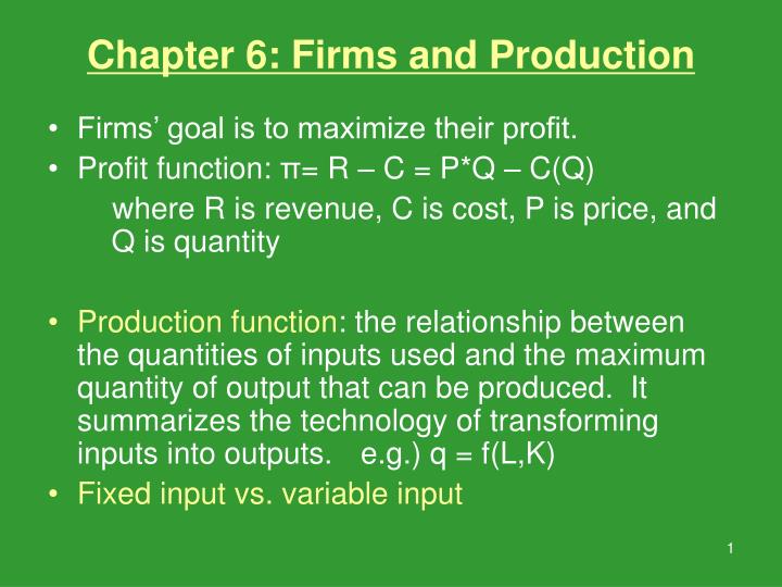
Chapter 6: Firms and Production. Firms’ goal is to maximize their profit. Profit function: π = R – C = P*Q – C(Q) where R is revenue, C is cost, P is price, and Q is quantity

E N D
Chapter 6: Firms and Production • Firms’ goal is to maximize their profit. • Profit function: π= R – C = P*Q – C(Q) where R is revenue, C is cost, P is price, and Q is quantity • Production function: the relationship between the quantities of inputs used and the maximum quantity of output that can be produced. It summarizes the technology of transforming inputs into outputs. e.g.) q = f(L,K) • Fixed input vs. variable input
Short-Run: At least one factor of production is fixed For production function: q = f(L,K) • Average product of labor (AP) = q/L • Marginal product of labor (MP) = △q/△L • AP increases when MP exceeds AP and decreases when MP is exceeded by AP.
Diminishing Marginal Returns(or diminishing marginal product) • If a firm keeps adding one more unit of input, holding all other inputs and technology constant, the extra output it obtains will become smaller eventually. • Why? • Too many workers per machine • Increases the cost of managing labors, etc.
Example: A Cobb-Douglas Function • Production Function: • Capital (K) is fixed. Only labor (L) is variable. • The marginal product of Labor is • The second derivative of q w.r.t. L is which is negative: Concave function. Assume that K is fixed at 100. Draw the production function and the marginal product of Labor.
Long-Run: All inputs are variable • Firms can vary input mix to achieve the most efficient production. • Isoquant: a curve that shows the efficient combinations of labor and capital that can produce a single level of output (similar to indifference curve) • Marginal Rate of Technical Substitution (MRTS): • the extra units of one input needed to replace one unit of another input that allows a firm to produce the same level of output • slope of an isoquant (i.e., )
MRTS and Marginal Products • By definition of isoquant: • To see the small change in q, totally differentiate an isoquant: Marginal increase in output from increasing L Change in L Total increase in output from increasing L by dL
Example: A Cobb-Douglas Function • Production Function: • Capital (K) is not fixed (long-run). • The marginal product of Labor is • The marginal product of Capital is The marginal rate of technical substitution (MRTS) is Draw the isoquant curve.
Returns to Scale • How much output changes if a firm increases all its inputs proportionately. • Long-run concept • Constant Returns to Scale (CRS): t * f(x1, x2) = f(tx1, tx2) • Increasing Returns to Scale (IRS): t * f(x1, x2) < f(tx1, tx2) • Decreasing Returns to Scale (DRS): t * f(x1, x2) > f(tx1, tx2)
Reasons for increasing or decreasing returns to scale • Increasing Returns to Scale (IRS): • A larger plant may allow for greater specializations of inputs. • Decreasing Returns to Scale (DRS): • Management problems may arise when the production scale is increased, e.g., cheating by workers. • Large teams of workers may not function as well as small teams.
For a Cobb-Douglas production function: • If we double all inputs, • CRS if • IRS if • DRS if
Productivity and Technical Change • Technical change: • Neutral technical change • q = A*f(L,K) • Non-neutral technical change • e.g. from labor-using to labor-saving
K Isoquants q = 30 → q = 45 q = 20 → q = 30 q = 10 → q = 15 L Illustration of Neutral Technical Change
Illustration of Non-neutral or Biased Technical Change K K-using or L-saving L-using or K-saving Original isoquants L