Download
1 / 18
180 likes | 291 Vues
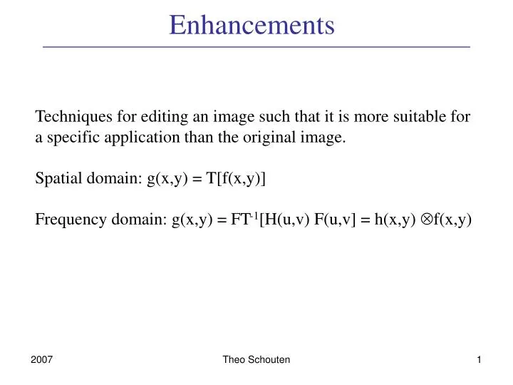
Enhancements. Techniques for editing an image such that it is more suitable for a specific application than the original image. Spatial domain: g(x,y) = T[f(x,y)] Frequency domain: g(x,y) = FT -1 [H(u,v) F(u,v] = h(x,y) f(x,y). Point processing. Gamma transformation: s = c r .

E N D
Enhancements Techniques for editing an image such that it is more suitable for a specific application than the original image. Spatial domain: g(x,y) = T[f(x,y)] Frequency domain: g(x,y) = FT-1[H(u,v) F(u,v] = h(x,y) f(x,y) Theo Schouten
Point processing Gamma transformation: s = c r Theo Schouten
Histogram Landsat image river Taag Histogram With histogram equalization we search for a T(r) that makes the histogram as smooth as possible. The T(r) that accomplishes that is: sk = round( L j=0k (nj / n) )with nk the number of pixels with gray level k, n the total number of pixels and L the number of gray levels. Theo Schouten
Examples Local contrast enhancement: g(x,y) =(x,y) + kM (f(x,y) - (x,y))/(x,y) Original Contrast stretched Hist. equalization Local histogram Local contrast Theo Schouten
Smoothing This is used for the blurring of an image: the removal of small details and the filling in of small gaps in lines, contours and planes, and also reduces the noise in an image. In the frequency domain smoothing becomes: G(u,v) = H(u,v)F(u,v) : low pass filter In the spatial domain smoothing is the removal of drastic changes by averaging the gray levels in a certain region with a positive weight. Theo Schouten
Smoothing Frequency domain Butterworth LPF: Hn(u,v)=1/(1+((u2+v2)/D0)2n ) the Exponential LPF: Hn(u,v)=exp(-(u2+v2)/D0 )n ) the Gaussian LPF: H(u,v)=exp( - (u2+v2) / 2 D02) Ideal LPF, the rings of especially the rivers can clearly be seen.Right image : Butterworth LPF with n=5. Here the ringing has decreased. Theo Schouten
Gaussian LPF Theo Schouten
Smoothing spatial domain A linear filter can be shown as a convolution mask: | 1 1 1 1 1 | |0 1 1 1 0| |1 2 3 2 1| |1 4 6 4 1| | 1 1 1 1 1 | |1 1 1 1 1| |2 4 6 4 2| |4 16 24 16 4|(1/25)| 1 1 1 1 1 | (1/21)|1 1 1 1 1| (1/81)|3 6 9 6 3| (1/256)|6 24 36 24 6| | 1 1 1 1 1 | |1 1 1 1 1| |2 4 6 4 2| |4 16 24 16 4| | 1 1 1 1 1 | |0 1 1 1 0| |1 2 3 2 1| |1 4 6 4 1| The 2 right filters are examples of separable filters, they can be executed as a convolution with (1/9) | 1 2 3 2 1 | respectively (1/16) | 1 4 6 4 1 | in the x direction, followed by a convolution in the y direction. The right filter is a poor approximation of the Gaussian function g(x,y) = c exp( (x2+y2) / 2 2), better ones are not separable. With a non-linear "rank" or "order-statistics" filter, the pixel values in the neighborhood are sorted according to increasing value, the value at a fixed position in the row is chosen to replace the central pixel. Choosing a value in the middle results in a so-called median filter. Theo Schouten
Examples mean and median image average filter median filter 9 9 9 0 0 0 . . . . . . . . . . . . 9 9 9 0 0 0 . 8 5 3 0 . . 9 9 0 0 . 9 0 9 0 0 0 . 8 5 4 1 . . 9 9 0 0 . 9 9 9 0 9 0 . 8 5 4 1 . . 9 9 0 0 . 9 9 9 0 0 0 . 9 6 4 1 . . 9 9 0 0 . 9 9 9 0 0 0 . . . . . . . . . . . . Original 5x5 mean 5x5 median 20% impulse noise 5x5 mean 5x5 median Theo Schouten
Noise models Theo Schouten
Noise models (2) Theo Schouten
Sharpening This is used to bring fine details to the front of the image and to sharpen the edges of objects. High Pass Filter: G(u,v) = H(u,v) F(u,v). ideal HPF: H(u,v) = 1 if (u2+v2) > D and 0 otherwise, see fig. 4.24 Butterworth HPF: H(u,v) = 1/(1+D/ (u2+v2) )2n, see fig. 4.25Exponential HPF: H(u,v) = exp(- D/ (u2+v2) )nGaussian HPF: H(u,v) = 1- exp( - (u2+v2) / 2 D02) see fig. 4.26 Theo Schouten
Examples combinations Here an example from High Frequency Emphasis, where the third order Butterworth HPF is added to the original image using the proportion 0.7:1. Blur masking: I-LPF(I) The impact of fragments from the Shoemaker-Levy comet on Jupiter on July 19th 1994. Theo Schouten
Sharpening in the spatial domain Differences in the gray levels between pixels, often as an approximation of the derivative of the image function f(x,y): f(x,y) = ( f/ x, f/ y )( ( f/ x)2 + ( f/ y)2 ) results in the gradient image. In the simplest case, one discretely approximates: f/ x = f[x,y] - f[x-1,y] g( f[x,y] ) = | f/ x | + | f/ y | Other manners often used to determine the derivative are: |1 0| | 0 1| |-1 -1 -1| |-1 0 1| |-1 -2 -1| |-1 0 1||0 -1| |-1 0| | 0 0 0| |-1 0 1| | 0 0 0| |-2 0 2| | 1 1 1| |-1 0 1| | 1 2 1| |-1 0 1| Roberts Prewitt Sobel Prewitt and Sobel take more pixels into account and are thus less sensitive to noise. Theo Schouten
Sobel Original Simple derivative Sobel Gausian Theo Schouten
Laplacian Other sharpening operators are derived from the Laplacian: 2 f(x,y) = 2f/ x2 + 2f/ y2 Discretely, one can use masks: |-1 -1 -1| | 0 -1 0|(1/9) |-1 8 -1| or (1/5) |-1 4 -1| |-1 -1 -1| | 0 -1 0| Theo Schouten
Moon Theo Schouten
Whole body bone scan Theo Schouten