Download
1 / 25
260 likes | 465 Vues
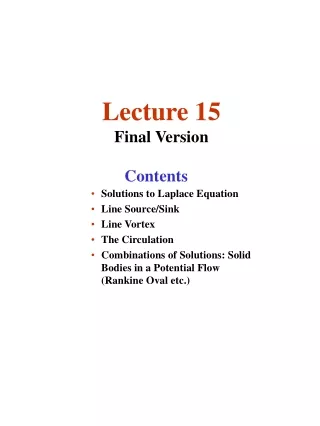
Lecture 15 Final Version. Contents. Solutions to Laplace Equation Line Source/Sink Line Vortex The Circulation Combinations of Solutions: Solid Bodies in a Potential Flow (Rankine Oval etc.). What Did We Do In Last Lecture?. Flow Around a Corner of Arbitrary Angle.

E N D
Lecture 15Final Version Contents Solutions to Laplace Equation Line Source/Sink Line Vortex The Circulation Combinations of Solutions: Solid Bodies in a Potential Flow (Rankine Oval etc.)
What Did We Do In Last Lecture? Flow Around a Corner of Arbitrary Angle One can interpret real part, R(x,y), of complex function, F(z), as velocity potential and imaginary part, I(x,y), as stream function of a two-dimensional flow. Derivative, F’=u-iv, corresponds to complex conjugate of velocity, u+iv.
We learnt that in inviscid, irrotational and incompressible flow Laplace equation determines flow field. For instance, in 2D all that is required is to solve: SOLUTIONS TO LAPLACE EQUATION (1) subject to boundary conditions (usually no flow through a solid boundary) obtained when a body (e.g. an aerofoil) is placed in a flow which is uniform infinitely far upstream.. • To satisfy boundary conditions, one often constructs a composite solution. Note that if are solutions to Eq. (1) then function is also a solution since: (2)
In general then, if where are each solutions to Laplace equation, so must be Continued … • This process of constructing a solution is known as LINEAR SUPERPOSITION. Functions , are usually well-known solutions to Laplace equation and are ‘building bricks’ of a composite solution. We construct a solution according to Eq. (2), finding necessary constants Ai such that boundary conditions are satisfied.
Some useful solutions to the Laplace Equation as examples • We now identify some useful solutions to Laplace equation. Remember that for a potential function to be a solution to Laplace equation velocity must satisfy conditions of zero vorticity and imcompressibility (the mass-continuity equation). • If fluid is incompressible and because we are dealing with two-dimensional flows, then there must also exist a stream function. Below we will identify both the velocity potential, , and the stream function, , for particular flows.
Paralell to the x-axis…. Example: Uniform Flow (Revision, see earlier examples!) Need to project free stream velocity onto radial and circumferential unit vector! Minus sign mathematically negative sense, i.e. clockwise In cartesians ... In polar coordinates ... • Have already seen in previous example that this flow has zero vorticity and that it satisfies the mass-continuity equation. • We found that velocity potential and stream function are... Velocity Potential Stream Function In cartesians ... In polar coordinates ...
Suppose z-axis were a sort of thin-pipe manifold through which issued fluid at a total rate Q uniformly along its length b. Looking at xy plane, we would see a cylindrical outflow or line source as sketched below. If flow is perfectly uniform then flow speed is entirely in radial direction, i.e. there is no circumferential velocity. Example: Line Source/Sink Questionsand Solutions: (Q1) Determine radial flow velocity ur as function of the radial coordinate r. (A1) Apply mass-continuity to a cylindrical control volume of radius r which has source as its centre line. Surface area of control volume through which fluid has to pass is... Since, ... Area x Flow Velocity = Volume Flow Rate Through Area one gets... (1) Will need this repeatedly. Keep this result in mind! :Source Strength; Volumetric flow rate (Q) per unit length and divided by
(Q2) Is this an irrotational flow? Think about deformation of fluid elements as they move away from the origin ... Continued... (A2) Need to verify that vorticity is zero. In polars, vorticity is ... (2) Substituting in values for radial and azimuthal velocity gives, ...
(Q3) Is mass-continuity satisfied? (A3) Evidently it will be satisfied from our derivation of radial and circumferential velocity. However, to show this formally, substitute these into mass-continuity equation. In polars mass-continuity is ... Continued... (3) Note symmetry / similarity of Eq. (2) and Eq. (3) in co- ordinates! Substituting in values for radial and azimuthal velocity gives, ... CONCLUDE: Because irrotational and mass continuity satisfied Laplace equation must be satisfied ... … everywhere in plane EXCEPT at origin, location of source, where radial flow speed, is infinite- Eq. (1) previous slide. Note: A sink is opposite of source - fluid is sucked into ‘hole’. Same formulation as for source is used except that source strength becomes -m
(Q4) Evaluate velocity potential and stream function! Continued... (A4) From their definitions, using polars ... Stream Function : (4a,b) Velocity Potential : (5a,b) …now integrate • From (4a) …now integrate From (4b) (6a) Compatibility required, as usual, and neglecting constant ... …now integrate • From (5a) From (5b) …now integrate Compatibility required, as usual, and neglecting constant ... (6b)
Velocity Potential Stream Function Continued... = ur • Again, note: • Stream function constant along streamlines (here in radial direction). • Lines of constant potential are perpendicular to streamlines • For what should be obvious reasons, polar coordinates have been used to determine the velocity potential and the stream function. • Can convert both into cartesian forms ...
Conversion of stream function and velocity potential into cartesian forms. Continued... • Suppose ‘red dot’ moves on circle around origin of xy coordinate system... • One has ... and • Added velocity components are... For our example circumferential velocity does not exis, hence... with... one gets ... (7a,b) And so ...
Velocity potential and stream function can either be found using integration of velocity components in Eq. (7a,b) from previous slide or by using solutions obtained earlier (Eq. (6a,b)) and performing a direct change of variables in polar-coordinate forms (remember that these are scalar quantities). Continued... Velocity Potential, Eq. (6b) Stream Function Eq. (6a) Change of Variables • Can use these forms to find velocity potential and stream function due to a source/sink which is not located at origin. If source/sink was located at (x0 , y0 ) then same analysis can be carried out using translated axes and following results apply:
Laplace Equation for velocity potential Example : Line Vortex • For irrotational, incompressible flow from previous example we can show that stream function also satisfies the Laplace equation, i.e. that... (1) • Recall... Hence, Eq. (1) equivalent to... Which is the statement that vorticity is zero! • This means that stream function for source/sink flow from previous example satisfies Laplace Eq.!!! (Recall, we started our previous example from velocity potential satisfying Laplace Eq.) • Hence, this stream function could represent velocity potential. • Therefore define new flow where roles of velocity potential and stream function have been swapped around, i.e ... Velocity Potential Stream Function where K is a constant (vortex strength). Velocity components are now easily found... Radial Velocity Component Circumferential Velocity Component
Continued... • This is a flow exclusively in tangential direction, with flow speed inversely proportional to (radial) distance from vortex centre. The larger the value of K the higher velocity at any particular radius r - this is why K is called vortex strength. Flow is akin to that seen around a plug hole… What would be a better representation of a flow near/down a plug hole? • Note that flow is not a rigid body motion with constant angular velocity and speed directly proportional to radial distance from axis of rotation! A B Along line AB one has 1/r velocity ‘decay’. Speed downwards on interval B0 and upwards on 0A. Velocity infinite at origin; of course this cannot happen in reality. In reality viscosity removes the singularity at origin.
AGAIN… Note from a physical standpoint that flow is IRROTATIONAL everywhere … except at origin where circumferential velocity is infinite and so is vorticity. Continued... Important here…. … to realize what irrotational means! … Put a piece of paper on our irrotational, potential vortex and watch it... What you observe as it goes around is... The EXCLAMATION MARK … … does NOT change its orientation in space as it moves around centre of the vortex! … This is because the flow is irrotational; its vorticiy is zero...!
For irrotational line vortex ‘exclamation mark did not rotate’ - in the sense of changing its orientation in space. Had it changed its orientation then flow would have been rotational. It is THIS rotation that vorticity deals with. THE CIRCULATION • Nevertheless, exclamation mark moved around centre of vortex. So there was some sort of rotary motion.This aspect of flow is connected with the CIRCULTATION. • For a region of flow... CIRCULATION IS DEFINED as the clockwise integral around the closed curve (that encloses the region) of the flow velocity component along the curve.
Hmhhh,… wouldn’t I expect this integral to be zero? • No it is not zero! Convince yourself by looking at the example ... (1) So, … integral (i.e. circulation) gives a finite value! Reason is that plus/minus signs always appear in such combinations that one always adds up (positive) terms! • Note, the larger u and v (i.e. the faster I move around curve) the larger circulation. • Similar sums as above in Eq.(1) could be written down for line vortex... • Circulation for line vortex will be constant no matter around which one of the circular streamlines I integrate. Velocity decrease as 1/r but circumference of circle increases proportional to r.
Two slides ago where we defined circulation we had… Continued... • So, then... (A) • For velocity potential one has: ! • Hence, ... Total Differential, 1st year Maths • So, then, ... Circulation only depends on values of velocity potential at start and end points of the path along which we integrate!
OK,… Then let’s calculate the circulation for our line vortex and for our source! (i) ForLINE VORTEX the velocity potentialwas found to be ... As we move along curve C surrounding the line vortex the angle changes as... Hence,... (ii) ForLINE SOURCE the velocity potentialwas found to be ... When we move along curve C surrounding line source then radius... Hence,...
NOTES: • Value of circulation does not depend on the shape of closed curve, C. To find results above, we could chose a circular or non-circular path round the vortex (i) and source (ii). Continued... • In general, value of circulation denotes net algebraic strength of all vortex filaments contained within the closed curve. This can be seen by re-writing the line integral into a surface integral using Stokes theorem... • Circulation is an important concept in fluid mechanics: it is circulation which (together with onset of flow speed) develops lift (Magnus Force) on a spinning cylinder, spinning cricket ball and an aerofoil section. • In potential flow, line vortex is used to model circulation that occurs in real life. • Use of word ‘Circulation’ to label integral used for its definition is slightly misleading. • It does not necessarily mean that fluid elements are moving around in circles within this flow field! • Rather, when circulation exist it simply means that line integral is finite. • For example, if airfoil below is generating lift the circulation taken around a closed curve enclosing the airfoil will be finite, although the fluid elements are by no means executing circles around the airfoil (as clearly seen from streamlines sketched in figure). Simplified version of ‘Wing Example’ on shown on left...
COMBINATIONS OF SOLUTIONS: SOLID BODIES IN A POTENTIAL FLOW • Recall: Can use PRINCIPLE OF SUPERPOSITION for velocity potential. • In addition, have shown that for incompressible, irrotational flow, stream function also satisfies Laplace Eq. So can similarly construct flow solutions by combining S.F. associated with uniform flow, source/sink flow and line-vortex flow. • In fact, we will almost exclusively use stream function here because we are interested in pattern of streamlines; once we find stream function, we can use fact that it is constant along streamlines to plot out streamlines. Uniform Flow and Source: THE RANKINE BODY What happens if we combine... ? (1) Cartesian Coordinates: (2) Polar Coordinates: • (1)/(2) represent complete descriptions of flow field. But what does it look like?... • To graph lines of constant , first look for STAGNATION POINTS. There ... Thus, both velocity components must be zero… Differentiate to get expressions for velocity components ...
Cartesian Coordinates: Continued... (3) (4) • For v=0 Eq. (4) requires ... ...with this Eq. (3) gives... STAGNATION POINT at • Polar Coordinates: and Since m, r positive choose... to get a solution for STAGNATION POINT at
In both cases same location for Stagnation Point ... Continued... Cartesian Coordinates Polar Coordinates We repeated ourselves to demonstrate that either coordinate system can be used. In general choose the one that makes the analysis easiest. • Now use for distance between origin and stagnation point: • Find S.L. that arrives at stagnation point and divides there. Using ... along this S.L., use a known point - the stagnation point - to evaluate constant. With Eq (2) from above ... where suffix s denotes ‘along particular streamline through stagnation point’. • Streamline found by equatingEq (2) to the constant and rearranging... (5)
Plotting stagnation streamline: Continued... • Stagnation streamline defines shape of (imaginary) solid half-body which may be fitted inside streamline boundary; remember flow does not cross streamline … or solid boundary. Call this special S.L. SURFACE STREAMLINE. • Body shape named after Scottish engineer W.J.M. Rankine (1820-1872). • Now only have stagnation/surface. To get other S.L.’s, choose point, determine constant for S.L. through point and then sketch particular S.L. through this point by compiling a table as above.