Download
1 / 15
150 likes | 264 Vues
Simulations of eastern Pacific climate using a new regional coupled ocean-atmosphere model. Shang-Ping Xie, Yuqing Wang, Haiming Xu, Toru Miyama, Simon deSzoeke, Richard Justin Small. Why build a regional coupled model ?.

E N D
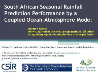
Simulations of eastern Pacificclimate using a new regional coupled ocean-atmosphere model Shang-Ping Xie, Yuqing Wang, Haiming Xu, Toru Miyama, Simon deSzoeke, Richard Justin Small
Why build a regional coupled model ? • To isolate the impact of regional coupled processes from external coupled processes. • To allow the use of high resolution and more expensive physical schemes in the area of interest. • Currently this model produces hindcasts with forcing from reanalysis products • -could be extended to future simulations (‘forecasts’) using global coupled climate models as forcing.
IPRC Regional Ocean-Atmosphere Model (iROAM) on ES Atmosphere: IPRC-RAM 0.5°×0.5°, L 28 Fig. 1 GFDL Modular Ocean Model 2 0.5°×0.5°, L 30 Forced by NCEP reanalysis Interactive Ocean spin-up Coupled ‘90 – ‘95 96 – 03
IPRC-RCM MM5 Model Physics – IPRC RCM and MM5 Scheme Authors Scheme Authors Primitive equations Hydrostatic Sigma Nonhydrostatic Sigma Boundary layer 1.5 level TC (K-) Langland-Liou (1996) Ri dependent+ Non-local Hong And Pan (1996) Surface layer TOGA-COARE Fairal (1996) Microphysics Wang 2001 Goddard Lin et al 1983 Radiation 7 bands LW 4 bands SW Edwards and Slingo 1996 Sun+Rikas1996 Rapid Radiative Transfer model Mlawer et al 1997 Cumulus Mass-flux CAPE Tiedke 1989 Gregory et al 2000 Kain-Fritsch Kain-Fritsch 1993 Land – surface processes Biosphere-Atm Transfer Dickenson 1993 Default
IROAM OBSERVATIONS TMI Fig. 2. Precipitation (mm/day, color), SST (° C, contour) and 10 m winds (vectors). Annual mean in IROAM (left) and in satellite observations (top right – SST and precip from TMI, bottom right: CMAP precip and OISST, winds from QuikSCAT). CMAP
Fig. 3 Annual cycle at 125-95 W.SST (° C, color), precipitation (> 2.5 mm/day shaded) and 10 m winds. OBSERVATIONS IROAM
Fig. 4. Cloudiness, SST & Wind (annual-mean) iROAM COADS
Fig. 5. Cloudiness, SST. Left: IROAM, Right: observed. (annual cycle between 110° W and 90° W)
NINO3 in model and observations HadSST MOM2 IROAM
Vertical ocean sections at 95 W 400 m depth U and pot. temp IROAM U 10cm/s U 10cm/s Johnson et al Johnson et al T IROAM
Vertical section at the equator: temperature and currents IROAM Johnson et. al. 2002
TIWs in IROAM IROAM produces TIW variability on the Equatorial front but the wavelengths and particularly periods are too short. This may be due to the weak front (baroclinicity) in IROAM which affects TIWs (Yu and McCreary 1995), or due to incorrect shear.
Sections at 95W, Sep 2001V and potential temperature IROAM RCM EPIC EPIC2001
Sections at 95W, Sep 2001: temp and liquid water RCM IROAM IROAM EPIC 2001
Discussion • We welcome collaboration: • Using observations to help the model • Using model to interpret observations