Download
1 / 22
260 likes | 441 Vues
Numerical Modeling of Climate. Hydrodynamic equations: 1. equations of motion 2. thermodynamic equation 3. continuity equation 4. equation of state 5. equations that govern water vapor, phase change, and latent heat. 6. conservation equations of various scalars.

E N D
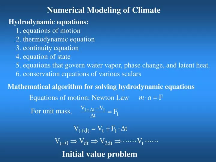
Numerical Modeling of Climate Hydrodynamic equations: 1. equations of motion 2. thermodynamic equation 3. continuity equation 4. equation of state 5. equations that govern water vapor, phase change, and latent heat. 6. conservation equations of various scalars Mathematical algorithm for solving hydrodynamic equations Equations of motion: Newton Law For unit mass, Initial value problem
Numerical simulation of climate: Using mathematical algorithms to solve a set of governing equations to predict the future state of the atmosphere based on the data of the past and present state of the atmosphere. Discretizing governing equations onto model grids Specifying surface conditions or coupling atmospheric model to oceanic model and land surface model
Historical background British scientist L. F. Richardson Weather Prediction by Numerical Process, 1922 Richardson estimated that a work force of 64,000 people would be required just to keep up with the weather at a global basis. But Richardson did not make a successful numerical forecast. Filtering meteorological noises American meteorologist J. G. Charney, 1948 Geostrophic and hydrostatic approximations Quasi-geostrophic model, 1950, the first numerical forecast
Akira Kasahra at the University of Chicago made the first numerical forecast of hurricane movement 1957. In the 50s, people are optimistic about numerical weather forecast • Global observational network of the atmosphere has been established, which can provide more accurate initial fields. • Great success of numerical calculation in other fields, such as calculating the trajectories of planetary orbits and long-range missals. • The accuracy of numerical forecast improved dramatically during the 60s, 70s, and 80s. • But unfortunately, improvement slowed nearly to a • standstill beginning around 90s. Why?
Challenges of numerical simulation of climate • Insufficient observations – leading to inaccurate initial conditions; • Chaotic nature of the atmospheric and oceanic system; • Inherent deficiency of numerical models with limited resolution that fails to resolve sub-grid physical processes.
1. Initial conditions a. Traditional approach: objective analysis and data initialization x x x 1. Objective analysis: Irregular observational data is converted onto regular model grid points using certain interpolation schemes. Such objectively analyzed data may contain noise . 2. Data initialization: Objectively analyzed data are further modified in a dynamically consistent way. 3. Data assimilation: Separate objective analysis and data initialization are combined together into an integrated one to obtain a best estimate of the state of the atmosphere at the analysis time using all available information.
2. Chaotic nature of the atmospheric and oceanic system: Sensitive dependence on initial conditions, butterfly effect Edward N. Lorenz (a professor at the MIT) equations: Round off 0.832479 to 0.832 Chaotic system
t=30 t=30 t=0 t=0 Lorenz attractor The Lorenz attractor starting at two initial points that differ only by of initial position in the x-coordinate. Initially, the two trajectories seem coincident, but the final positions at t=30s are no longer coincident.
This scenario can really wreak havoc with hurricane track forecast
Ensemble simulation: (1) one model, different initial conditions (2) same initial condition, many models IPPC simulations
Ensemble Prediction Ensemble forecasting is a method used by modern operational forecast centers to account for uncertainties and errors in the forecasting system which are crucial for the prediction errors due to the chaotic nature of the atmospheric dynamics (sensitive dependency on initial conditions). Many different models are created in parallel with slightly different initial conditions or configurations. These models are then combined to produce a forecast that can be fully probabilistic or derive some deterministic products such as the ensemble mean.
3. Limited model resolution: how to represent sub-grid physical processes in models turbulence clouds Grid size of climate models: ~50 – 100/200 km ~10 km ~100 m – a few km
Scale (km) 1800 180 18 1.8 0.18 0.018 Van de Hoven (1957) Parameterization Representation of sub-grid physical processes in terms of model resolved quantities
Hurricane boundary layer turbulent processes Turbulent transport turbulence Warm ocean Do the parameterizations realistically represent the energy transported by the turbulence in numerical models?
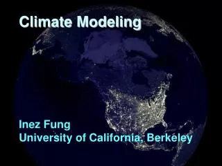
Climate modeling State-of-the-art climate models now include the interactive representations of the ocean, the atmosphere, the land, the hydrologic and cryospheric processes, terrestrial and oceanic carbon cycles, and atmospheric chemistry.
Physical parameterization 1. Boundary layer process (turbulence) 2. Moist convection process 3. Cloud microphysics and precipitation 4. Radiation
Atmospheric model components: 1. Initialization package 2. Dynamic core 3. A suite of parameterizations 4. Coupler with other components in the climate system, such as ocean, land, sea ice, … 5. Post-processing package
National Center for Atmospheric Research Community Earth System Model
NCAR CESM 1.0 http://www.cesm.ucar.edu/models/cesm1.0/