Download
1 / 15
150 likes | 294 Vues
Slides accompanying Greenhouse gas emission targets for limiting global warming to 2°C Meinshausen, M., Meinshausen, N., Hare, W., Raper, S. C. B., Frieler, K., Knutti, R., Frame, D. J. & Allen, M. Nature (2009).

E N D
Slides accompanyingGreenhouse gas emission targets for limiting global warming to 2°C Meinshausen, M., Meinshausen, N., Hare, W., Raper, S. C. B., Frieler, K., Knutti, R., Frame, D. J. & Allen, M. Nature (2009).
Figure 1 | Joint and marginal probability distributions of climate sensitivity and transient climate response (TCR).a, Marginal PDFs of climate sensitivity; b, marginal PDFs of TCR; c, posterior joint distribution constraining model parameters to historical temperatures, ocean heat uptake and radiative forcing under our representative illustrative priors. For comparison, TCR and climate sensitivities are shown in panel c for model versions that yield a close emulation of 19 CMIP3 AOGCMs (white circles)16.
Figure 2 | Emissions, concentrations and 21st century global mean temperatures. a, Fossil CO2 emissions for IPCC SRES22, EMF-2121 scenarios and a selection of EQW25 pathways analyzed here; b, greenhouse gas emissions, as controlled under the Kyoto Protocol; c, median projections and uncertainties based on our illustrative default case for atmospheric CO2 concentrations for the high SRES A1FI22 and the low HALVED-BY-205030 scenario, which halves 1990 global Kyoto-gas emissions by 2050; d, total anthropogenic radiative forcing; e, surface air global mean temperature; f, maximum temperature during the 21st century versus cumulative Kyoto-gas emissions for 2000-2049.
Figure 3 | The probability of exceeding 2°C warming versus CO2 emitted in the first half of the 21st century.a, Individual scenarios’ probabilities of exceeding 2°C for our illustrative default (small dots) and smoothed (least squares polynomial fits) probabilities for all climate sensitivity distributions (numbered lines, cf. Fig. 1a). The proportion of CMIP3 AOGCMs26 and C4MIP carbon cycle8 model emulations exceeding 2°C is shown as black dashed line. Coloured areas denote the range of probabilities of staying below 2°C in IPCC AR4 terminology – with the extreme upper distribution (12) being omitted; b, total CO2 emissions already emitted3 between 2000 and 2006 (grey area) and those that could arise from burning available fossil fuel reserves, and from landuse activities between 2006 and 2049 (median and 80% ranges, Methods).
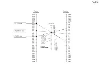
Figure S1 | Probabilities of exceeding 2°C for various emission indicators:a, cumulative Kyoto-gas emissions 2000-2049; b, 2050 year Kyoto-gas emissions: c, 2020 Kyoto-gas emissions. Otherwise as Figure 3 in the main part of the paper. In panel c the wide vertical spread of individual scenarios’ exceedance probabilities (dots) indicates that 2020 emissions are a relatively poor indicator for maximum warming. This contrasts with 2050 Kyoto-gas emissions (b), for which the narrow vertical spread of individual scenarios’ exceedance probabilities suggests that this indicator is well suited for the chosen class of scenarios. The dashed vertical lines in panel b indicate halved 1990 Kyoto-gas emissions and the bold line indicates the respective range of exceedance probabilities derived from our default constraining as well as the emulation of other studies’ climate sensitivity distributions.
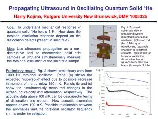
Figure S2 | Observations and constrained model results for temperatures and ocean heat content changes.a, Modelled average surface temperatures using the illustrative default case and observed2 data with 95% uncertainty range for northern hemisphere ocean; b, northern hemisphere land; c, southern hemisphere ocean; d, southern hemisphere land; e, the global average; f, Modelled and observed4,5 changes in ocean heat content up to 700m depth. The regional temperatures and the linear trend of ocean heat uptake4 over 1961 to 2003 were used to constrain the climate model parameter space. The MAGICC 6.0 results based on our illustrative default are shown in blue. The agreement between observed and modelled ocean heat uptake up to 300m or 3000m depth5 is similar as shown here for 700m. Fig S2a-d
Figure S3 | Joint distribution of seven key MAGICC parameters, as example of the 82-dimensional parameter space we constrained.a-g, Histograms of parameters are provided in the diagonal, and 2000 randomly drawn parameter sets are indicating the joint distributions (illustrative default) between any two parameters in the off-diagonal scatter plots. Parameter sets that were calibrated to emulate 19 CMIP3 AOGCMs are provided as red dots in the off-diagonal scatter plots of the parameters climate sensitivity (a), ocean vertical diffusivity (b) and equilibrium land-ocean warming ratio (c).
Figure S4 | Sensitivity test for the shape parameters of the EQW emission pathway ensemble. Probability of exceeding 2°C warming as a function of cumulative total CO2 emissions are shown for different sets of EQW pathways.
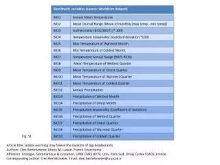
Figure S5 | Comparison of key emission scenario characteristics between EQW and multi-gas IPCC SRES, EMF-21 scenarios.a, cumulative Kyoto-GHG emissions between 2000 and 2049; b, cumulative Kyoto-GHG emissions between 2000 and 2099; c, single-year Kyoto-GHG emissions in the year 2050; d,e,f, same as a,b,c but for fossil & industrial CO2 emissions. SRES and EMF-21 scenarios are shown as red, orange and dark blue dots and the default EQW pathway ensemble used in this study is shown as bright blue dots in off-diagonal plots and histograms on the diagonal.
Figure S6 | Regression of CO2 concentrations in year 2100 to net total radiative forcing. a, CO2 concentrations vs. total radiative forcing for emission scenarios used in this study (small colored dots), and the stabilization scenarios (grey dots) including the linear regression (black line) as shown in Fig. 3.16 of Working Group III, IPCC AR419; b, CO2 concentrations vs. non-CO2 radiative forcing in year 2100, including the regression line from a. The linear regression shown in a is not linear when plotted in panel b due to the non-linear concentration to forcing relationship of CO2. The IPCC AR4 WGIII regression hence includes the implicit assumption of higher non-CO2 forcing, the more CO2 concentrations are reduced below about 475ppm (cf. black bold line bending upwards towards low concentration levels in panel b). Another difference of our study is that – on average – our results suggest lower non-CO2 radiative forcing contributions in 2100 than implied by the WGIII regression line (see text).