Download
1 / 53
530 likes | 782 Vues
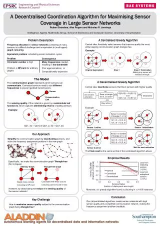
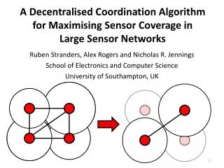
A Decentralised Coordination Algorithm for Maximising Sensor Coverage in Large Sensor Networks. Ruben Stranders , Alex Rogers and Nicholas R. Jennings School of Electronics and Computer Science University of Southampton, UK. This work is about constructing large sensor networks.

E N D
A Decentralised Coordination Algorithm for Maximising Sensor Coverage in Large Sensor Networks Ruben Stranders, Alex Rogers and Nicholas R. Jennings School of Electronics and Computer Science University of Southampton, UK
This work is about constructing large sensor networks Frequency assignment problem Maintain good sensor quality Efficient (polynomial time) algorithms
These networks consist of many resource constrained sensing devices Sensor 1. Deployment
These networks consist of many resource constrained sensing devices Radio Link 2. Construct communication network
Sensing quality is modelled by a submodular set function 1 1 3 3 2 Q({1, 3}) – Q({1}) ≥ Q({1, 2, 3}) – Q({1, 2}) Models the diminishing returns of adding a sensor
Sensing quality is modelled by a submodular set function 1 1 3 3 2 • Examples (Guestrin 2005): • Mutual Information • Area Coverage • Entropy
Frequency allocation is one of the key challenges Equivalent to (multi-agent) graph colouring Communication graph
Frequency allocation is one of the key challenges Communication graph
Frequency allocation is one of the key challenges Garbled Reception Colouring the communication graph is not sufficient
Frequency allocation is one of the key challenges We need to consider the conflict graph (Square of the communication graph)
Frequency allocation is one of the key challenges We need to consider the conflict graph (Square of the communication graph)
The frequency allocation is one of the key challenges Multi-agent graph colouring occurs often in sensor networks e.g. Coordination of sense/sleep cycles
Frequency allocation is a difficult challenge for two reasons 1. Might need many frequencies Reduced bandwidth Poor approximations 2. NP-hard problem or Requires lots of resources
Specifically, our approach is to make the communication graph triangle-free Triangle-free Graph (K3-minor free) Arbitrary Graph Colourable with threecolours Might need many colours Colouring is NP-hard Colouring can be foundin linear time
Specifically, our approach is to make the communication graph triangle-free Triangle-free Graph (K3-minor free) Arbitrary Graph Colourable with threecolours Might need many colours Colouring is NP-hard Colouring can be foundin linear time
Specifically, our approach is to make the communication graph triangle-free Triangle-free Graph (K3-minor free) Colourable with threecolours Colouring can be foundin linear time
Specifically, our approach is to make the communication graph triangle-free Triangle-free Graph (K3-minor free) Square of Triangle-free Graph Conflict Graph Communication Graph Colourable with threecolours Colourable with six colours Colouring can be foundin linear time Colouring is easy
However, by deactivating sensors, we lose sensing quality Sensor coverage area
However, by deactivating sensors, we lose sensing quality Sensing quality is given by submodular function
Maximising quality while simplifying frequency allocation is still NP-hard Maximise sensing quality subject to graph being triangle-free Maximising submodular function subject to p-independence constraint
Therefore, we developed two efficient approximate algorithms Arbitrary Graph Triangle-free Graph
The centralised algorithm iteratively selects sensors that improve quality Each iteration, activate the sensor that: • Maximises quality increase without • Creating a triangle
The centralised algorithm iteratively selects sensors that improve quality
The centralised algorithm iteratively selects sensors that improve quality Step 1
The centralised algorithm iteratively selects sensors that improve quality Step 2
The algorithm terminates when no remaining sensor can be activated Can’t add: creates triangle! Can’t select any more sensors.
The algorithm terminates when no remaining sensor can be activated Done Can’t select any more sensors.
The centralised algorithm achieves at least 1/7th of the optimal quality Greedy Optimal This follows from submodularity and p-independence
The centralised algorithm achieves at least 1/7th of the optimal quality p-independence system Need to remove at most p sensors after adding an arbitrary sensor to retain triangle-freeness
The centralised algorithm achieves at least 1/7th of the optimal quality p-independence system Need to remove at most p sensors after adding an arbitrary sensor to retain triangle-freeness
The centralised algorithm achieves at least 1/7th of the optimal quality p-independence system Need to remove at most p sensors after adding an arbitrary sensor to retain triangle-freeness p = 6
The centralised algorithm achieves at least 1/7th of the optimal quality Greedily maximising submodular function subject to p-independence constraint QG ≥ 1/(1+p) Q* (Nemhauser, 1978) QG ≥ 1/7 Q*
Using similar techniques, we created a decentralised algorithm
Using similar techniques, we created a decentralised algorithm Central Idea In every triangledeactivate the sensor that blocks the two with highest quality 1 2 3 4
Using similar techniques, we created a decentralised algorithm Sensors activate themselves asynchronously 1 2 3 4
Sensors check if activating themselves block sensors with higher quality Sensor checks if it is part of a triangle 1 2 3 4
Sensors check if activating themselves block sensors with higher quality Is the sensor part of a triangle? 1 2 Yes: we have to deactivate at least one of these No: the sensor can remain active 3 4
Sensors check if activating themselves block sensors with higher quality Sensor checks if its contribution is smaller than that of the other two 1 2 Q({1, 2}) ≤ Q({2, 3}) 3 4 and Q({1, 3}) ≤ Q({2, 3})
Sensors check if activating themselves block sensors with higher quality Sensor checks if its contribution is smaller than that of the other two 1 2 ✓ Q({1, 2}) ≤ Q({2, 3}) 3 4 and ✓ Q({1, 3}) ≤ Q({2, 3})
Sensors check if activating themselves block sensors with higher quality Sensor checks if its contribution is smaller than that of the other two 1 2 If so, it deactivates itself 3 4
Sensors check if activating themselves block sensors with higher quality 1 2 3 4
Sensors check if activating themselves block sensors with higher quality 1 2 ✘ Q({2, 3}) ≤ Q({3, 4}) 3 4 and ✓ Q({2, 4}) ≤ Q({3, 4})
Sensors check if activating themselves block sensors with higher quality 1 2 3 4
The algorithm terminates when the sensor is no longer part of a triangle Done
Both algorithms efficiently compute a triangle-free network Original
Both algorithms efficiently compute a triangle-free network Centralised
Both algorithms efficiently compute a triangle-free network Decentralised
To evaluate the algorithms, we simulated sensor deployments 0 0 0 Unit square environment 1 R 300 sensors 0 1
Both algorithms provide >70% sensing quality of the original deployment Loss from restricting solution ( < 20% ) Sensing Quality Loss from suboptimal solution ( < 10% ) Sensing Radius