Download
1 / 29
290 likes | 479 Vues
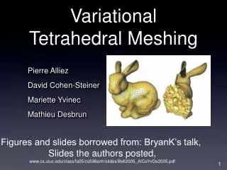
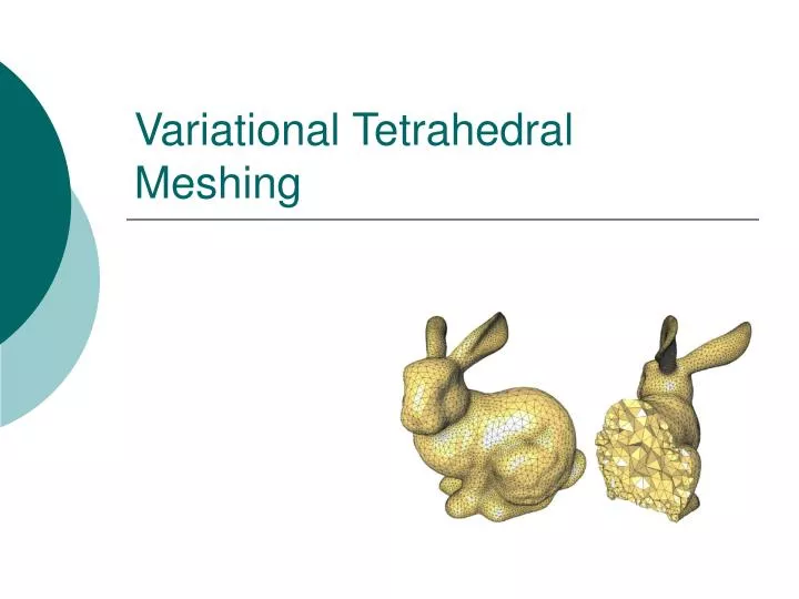
Variational Tetrahedral Meshing. Objective. Given a watertight, non-intersecting manifold triangle mesh Produce tet mesh with well-shaped tets Various tet shape metrics [Shewchuck] Radius ratio is “fair”, radius-edge is not. Other Requirements. Sizing field. Previous Work.

E N D
Objective • Given a watertight, non-intersecting manifold triangle mesh • Produce tet mesh with well-shaped tets • Various tet shape metrics [Shewchuck] • Radius ratio is “fair”, radius-edge is not
Other Requirements • Sizing field
Previous Work • Laplacian Smoothing • Edge-based • Results in many poorly-shaped tets • Edge flipping • Can’t hurt, but can only do so much
Previous Work • Bubble Meshing
Background • Voronoi Tessellation
Background • Delaunay Triangulation • Dual of Voronoi Tessellation
Centroidal Voronoi Tessellations (CVTs) • Generators are centroids of Voronoi regions
Centroidal Voronoi Tessellations (CVTs) • Not unique
Applications of CVTs [Du et. al. 1999] • Compression, Clustering • Optimal Quadrature • Resource Placement (e.g. mailboxes)
Tilapia – a noble fish • Fun Fact: Taiwan Tilapia was selected by NASA as the first fish to be sent into outer space. Tilapia was chosen by biologists at NASA, as the optimum fish for possible aquaculture in space because this fish has the practical features that seldom occur all within the same fish species. -- Wikipedia
Quadrature Example • Estimate integral by finite sum: • Assuming function is Lipschitz…
Computing CVTs • Lloyd’s Method • New points are centroids of regions • Continuous version of K-means
CVTs for mesh smoothing [Du & Wang] • Optimizes the following functional • Important: For a given set of vertices, the VT produces the (globally) optimal connectivity! • i.e. the Voronoi regions about each vertex are the best decomposition of the domain • Hence we can alternate vertex and connectivity optimization
Optimal Delaunay Triangulations (ODT) • Optimizes the DT (not its dual VT) • Again, the DT is optimal just as before • Unlike CVT, these regions overlap
Alternating Optimizations • Fixing the vertices, the Delaunay Triangulation gives optimal connectivity • Fixing the Triangulation, we want to optimize the vertices
Optimizing Vertex Positions • Fix the triangulation and take gradient of functional w.r.t. vertex positions • Messy expression: • … fortunately, an equivalent geometric interpretation is more reasonable
Optimizing Vertex Positions • Geometric Equivalent: • … move the vertex to the volume-weighted average of the circumcenters of tets in the 1-ring
Basic Algorithm • While improvement needed • (1) Compute Delaunay Triangulation for the current vertices • (2) Update vertex positions
Sizing Field • So far, method produces uniform meshes • Can be modified to accommodate a desired edge length
Automatic Design of Sizing Field • Paper uses Local Feature Size (LFS) • Defined on the mesh surface • Minimum distance to the skeleton (medial axis) of the mesh
Local Feature Size • LFS is now defined on the boundary and must be propagated inward • Desire smooth, controllable gradation • Choose the maximal K-Lipschitz function that does not exceed LFS on the boundary
Sizing Field Propagation • Computed using Fast Marching Method [Sethian]