Download
1 / 25
290 likes | 644 Vues
Bivariate Correlation. Lesson 11. Measuring Relationships. Correlation degree relationship b/n 2 variables linear predictive relationship Covariance If X changes, does Y change also? e.g., height ( X ) and weight ( Y ) ~. Covariance. Variance

E N D
BivariateCorrelation Lesson 11
Measuring Relationships • Correlation • degree relationship b/n 2 variables • linear predictive relationship • Covariance • If X changes, does Y change also? • e.g., height (X) and weight (Y) ~
Covariance • Variance • How much do scores (Xi) vary from mean? • (standard deviation)2 • Covariance • How much do scores (Xi, Yi) from their means
Covariance: Problem • How to interpret size • Different scales of measurement • Standardization • like in z scores • Divide by standard deviation • Gets rid of units • Correlation coefficient (r)
Pearson Correlation Coefficient • Both variables quantitative (interval/ratio) • Values of r • between -1 and +1 • 0 = no relationship • Parameter = ρ (rho) • Types of correlations • Positive: change in same direction • X then Y; or X then Y • Negative: change in opposite direction • X then Y; or X then Y ~
Correlation & Graphs • Scatter Diagrams • Also called scatter plots • 1 variable: Y axis; other X axis • plot point at intersection of values • look for trends • e.g., height vs shoe size ~
6 7 8 9 10 11 12 Scatter Diagrams 84 78 Height 72 66 60 Shoe size
Slope & value of r • Determines sign • positive or negative • From lower left to upper right • positive ~
Slope & value of r • From upper left to lower right • negative ~
Width & value of r • Magnitude of r • draw imaginary ellipse around most points • Narrow: r near -1 or +1 • strong relationship between variables • straight line: perfect relationship (1 or -1) • Wide: r near 0 • weak relationship between variables ~
Weak relationship Strong negative relationship r near 0 r near -1 300 300 250 250 Weight Weight 200 200 150 150 3 3 6 6 9 9 12 12 15 15 18 18 21 21 100 100 Chin ups Chin ups Width & value of r
Strength of Correlation • R2 • Coefficient of Determination • Proportion of variance in X explained by relationship with Y • Example: IQ and gray matter volume • r = .25 (statisically significant) • R2 = .0625 • Approximately 6% of differences in IQ explained by relationship to gray matter volume ~
Guidelines for interpreting strength of correlation *from Statistics for People Who (Think They) Hate Statistics: Excel 2007 Edition By Neil J. Salkind
Factors that affect size of r • Nonlinear relationships • Pearson’s r does not detect more complex relationships • r near 0 ~ Peeps (Y) Stress (X)
Factors that affect size of r • Range restriction • eliminate values from 1 or both variable • r is reduced • e.g. eliminate people under 72 inches ~
Hypothesis Test for r • H0: ρ = 0 rho = parameter H1: ρ≠ 0 • ρCV • df = n – 2 • Table: Critical values of ρ • PASW output gives sig. • Example: n = 30; df=28; nondirectional • ρCV = + .361 • decision: r = .285 ? r = -.38 ? ~
Using Pearson r • Reliability • Inter-rater reliability • Validity of a measure • ACT scores and college success? • Also GPA, dean’s list, graduation rate, dropout rate • Effect size • Alternative to Cohen’s d ~
Evaluating Effect Size • Pearson’s r • r= ±.1 • r = ±.3 • r = ±.5 ~ • Cohen’s d • Small: d = 0.2 • Medium: d = 0.5 • Large: d = 0.8 Note: Why no zero before decimal for r ?
Correlation and Causation • Causation requires correlation, but... • Correlation does not imply causation! • The 3d variable problem • Some unkown variable affects both • e.g. # of household appliances negatively correlated with family size • Direction of causality • Like psychology get good grades • Or vice versa ~
Point-biserial Correlation • One variable dichotomous • Only two values • e.g., Sex: male & female • PASW/SPSS • Same as for Pearson’s r ~
Correlation: NonParametric • Spearman’s rs • Ordinal • Non-normal interval/ratio • Kendall’s Tau • Large # tied ranks • Or small data sets • Maybe better choice than Spearman’s ~
Correlation: SPSS • Data entry • 1 column per variable • Menus • Analyze Correlate Bivariate • Dialog box • Select variables • Choose correlation type • 1- or 2-tailed test of significance ~
Reporting Correlation Coefficients • Guidelines • No zero before decimal point • Round to 2 decimal places • significance: 1- or 2-tailed test • Use correct symbol for correlation type • Report significance level • There was a significant relationship between the number of commercials watch and the amount of candy purchased, r = +.87, p (one-tailed) < .05. • Creativity was negatively correlated with how well people did in the World’s Biggest Liar Contest, rS = -.37, p (two-tailed) = .001.
Correlation: Example • Analysis using the Pearson’s r correlation indicated that the there was moderately strong negative relationship between the number of work hours and the number of hours spent on extracurricular activities, but the relationship was not statistically significant, r = -.31, p (two-tailed) = .08. The R2 = .097, indicating that the relationship accounts for approximately 9.7% of the variance in the number of hours spent in each activity.