Download
1 / 75
770 likes | 1.19k Vues
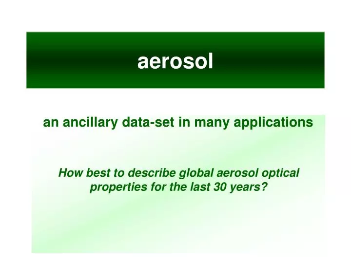
aerosol. an ancillary data-set in many applications How best to describe global aerosol optical properties for the last 30 years?. aerosols !. aerosol (‘small atmos.particles’) many sources short lifetime diff. magnitudes in size changing over time aerosol clouds

E N D
aerosol an ancillary data-set in many applications How best to describe global aerosol optical properties for the last 30 years?
aerosols ! • aerosol (‘small atmos.particles’) • many sources • short lifetime • diff. magnitudes in size • changing over time • aerosol clouds • aerosol chemistry • aerosol biosphere • aerosol aerosol highly variable in space and time ! rapid atmospheric ‘cycling’ ocean industry cities forest desert volcano
needs • global consistent data for all aerosol properties • AOD, SSA, g (amount, absorption, size) • satellite data … only deliver in part • limited spatial coverage (non-polar, darker) • usually only AOD … with assumptions • modeling … can deliver • but can it be trusted ? (even if constrained by satellite AOD pattern & component treatment) • data assimilation ? ! • MACC is not ready yet / hindcasts are too few
climatology • the next best thing • monthly 1x1 climatology for mid-visible aerosol properties of AOD, SSA and Angstrom ( g) • start with ‘one year’ (year 2000 or ‘current’) • median of 15 component models (no extremes) • enhance with quality AERONET data (merging) • extend spectrally • use simulation to scale back/forward in time • add altitude information (modeling or CALIPSO)
start with modeling • advantages • complete consistent (no data-gaps) • issues • as good as assumptions … the ‘tuning’ to observations • all relevant aerosol optical properties • aerosol optical depth (AOD) • single scattering albedo • Angstrom asymmetry factor annual aerosol optical depth at 550nm modeling
merge in AERONET data • merge • quality statistics of AERONET • onto • consistent background statistics by global modeling • NO satellite • NO grd in-situ AERONET modeling
the merging • combine point data on regular grid (1ox1o lon/lat) • extend spatial influence of identified sites with better regional representation • spatially spread valid grid ratios and combine • decaying over +/- 180 (lon) and +/- 45 (lat) • apply ratio field values (A) at site domains with distance decaying weights (B) corr. factors example: correction to model suggested AOD A B A*B ratio field site weight correction factor
merging results model merged AERONET 0.55mm • AOD • SSA • Ang
spectral extension • use the Angstrom to statify AOD into • AOD, f (fine-mode … particles > 0.5mm radius) • AOD, c (coarse-mode … part. < 0.5mm radius) • use SSA to identify dust size • when fine mode SSA falls below threshold • coarse mode spectral dependence is defined • sea-salt or dust (4 different sizes) • fine mode spectral dependence only for solar • g (from Angstrom) and SSA drop in near-IR
spectral samples – annual avg maps g AOD SSA • UV 0.4mm • VIS 0.55mm • n-IR 1.0mm • IR 10mm
extension in time • does NOT change with time • coarse mode • pre-industrial fraction of fine mode • use info on what is ‘anthropo’ from modeling • changes with time • stratospheric aerosol • anthropogenic fraction of the fine mode • back: ECHAM simulation with NIES emissions • forward: ECHAM runs with rcp scenarios
altitude • current distributions • total aerosol • CALIPSO version 2 • ECHAM • Separately for fine and coarse mode • ECHAM • next … CALIPSO version 3 • use (non-sphere) (=dust) for coarse • use total-(non-sphere) for fine
total AOD (550nm) by layer ECHAM 5 / HAM (model) CALIPSO vers.2 (obs)
aerosol climatology S. Kinne and colleagues MPI-Meteorology with support by AeroCom and AERONET
overview • aerosol in (global) climate modeling • (tropospheric) aerosol climatology • concept • column optical properties • altitude distribution • changes in time • link to clouds • some applications • further improvements
aerosols ! • aerosol (‘small atmos.particles’) • many sources • short lifetime • diff. magnitudes in size • changing over time • aerosol clouds • aerosol chemistry • aerosol biosphere • aerosol aerosol highly variable in space and time ! rapid atmospheric ‘cycling’ ocean industry cities forest desert volcano
aerosols ? • the radiation budget is modulated by clouds • so, what is all the fuss about aerosol ? • aerosol has a role in cloud formations • many clouds exist because of avail. aerosols • aerosol has an anthropogenic component • the impact on climate is highly uncertain and at times speculative (for indirect effects)
complex aerosol modules • they do exist - even in Hamburg ECHAM/HAM • they are useful … but often too expensive HAM calculations carry 27 tracers ! size optically active and relevant sizes
simplifications ? • simplified methods have been tried in the past • ignore aerosol • compensate with a radiation correction • simplify by ignoring fine-mode absorption • improve on the Tanre-scheme used in ECHAM IPCC 4AR simulations • a highly absorbing dust bubble over Africa • lack in seasonal feature (e.g. biomass) • now better simplifications are possible • matured complex aerosol module output • improved obs. constrains by remote sensing
new aero climatology goal • provide a simplified aerosol representation in global models for rapid estimates on aerosol direct & indirect effects on the radiation budget • establish aerosol optical properties (as they required for atmospheric radiative transfer) at sufficient resolution … in order to resolve regional variability and seasonality • whenever possible, tie climatology data to (quality) observations • establish via CCN (cloud condensation nuclei) or IN (ice nuclei) links to cloud properties
data sources • the available observables • ground based in-situ samples • satellite guesses • sun-/sky- photometry • the modeling world • data-constrained simulations • ensemble output
ground samples ? • issues • ground composition is not that of the column • samples are usually heated (less or no water) • monthly statistics example size absorption up quartile median low quartile
satellite data ? • issues • ancillary data needed • indirect reflection info requires information on aerosol absorption (usually assumed) and reflection contribution by other sources (such as surface or clouds) at high accurcay • limited information content • only AOD is retrieved and via AOD spectral dependency some information on size • limited coverage • land?, not with clouds, daytime, not polar, … • positives • spatial distribution statistics
seasonal AOD by satellites combining MODIS, MISR, AVHRR data
ground-based sun-photometry • advantages • direct AOD measurements • AOD and fine-mode AOD • other aerosol properties with sky-radiance data • size distribution (0.05mm < size bins < 15 mm) • single scatt. albedo (noise issue at low AOD) • issues • local … may fail to represent its region • daytime and cloud-free ‘bias’
global modeling • advantages • complete consistent (no data-gaps) • issues • as good as assumptions … the ‘tuning’ to observations • all relevant aerosol optical properties • aerosol optical depth (AOD) • single scattering albedo • Angstrom asymmetry factor annual aerosol optical depth at 550nm modeling
climatology concept • merge • quality statistics of AERONET • onto • consistent background statistics by global modeling • NO satellite • NO grd in-situ AERONET modeling
aerosol climatology • resolution and data content • processing steps • essential properties • temporal variations • link to clouds • first applications • further improvements
climatology products • global monthly 1x1 lat-lon maps • fine mode (radius < 0.5mm) properties • column AOD, SSA, g (… for each l) • altitude distribution • anthropogenic AOD fraction (1850 till 2100) • pre-industrial AOD fraction • coarse mode (radius > 0.5mm) properties • column AOD, SSA, g (… for each l) • altitude distribution • cloud relevant properties • CCN concentration (kappa approach) • IN concentration (coarse mode dust)
climatology details / steps • define global monthly maps of mid-visible aerosol column prop (AOD, SSA & Ang) • spread data spectrally to define AOD, SSA & g needed for radiative transfer simulations • add altitude information using active remote sensing from space and/or modeling • account for decadal (anthrop.) change using scaling data from aerosol component modeling • establish a (needed) link to cloud properties by extracting associated CCN and IN
column optical properties • concept combine • for mid-visible aerosol properties (0.55 mm) • for monthly (multi-annual) data • for a (1ox1o lon/lat) horizontal resolution • AeroCom model median maps • consistent and complete maps • median of a 15 model ensemble removes extreme behavior of individual models • quality data by sun-/sky-photometry networks • data of ~400 AERONET and ~10 Skynet sites
the merging • combine point data on regular grid (1ox1o lon/lat) • extend spatial influence of identified sites with better regional representation • spatially spread valid grid ratios and combine • decaying over +/- 180 (lon) and +/- 45 (lat) • apply ratio field values (A) at site domains with distance decaying weights (B) corr. factors example: correction to model suggested AOD A B A*B ratio field site weight correction factor
merging results model merged AERONET 0.55mm • AOD • SSA • Ang
merging note: low ssa at low AOD are unreliable
merging results model merged AERONET 0.55mm • AOD • SSA • Ang other .. fine-mode anthropogenic fraction kappa dust size
spectral extension (1) • concept • split AOD contribution by small & large sizes • fine-mode size (radii < 0.5um) • coarse-mode size (radii > 0.5um) • apply the Angstrom for total aerosol … with • pre-defined fine-mode Angstrom at function of ‘low clouds’: Ang,f = [1.6 moist … 2.2 dry] • fixed coarse-mode Angstrom: Ang,c = 0.0 • coarse mode (spectr. dep. properties) prescribed • apply the single-scatt. albedo for total aerosol • sea-salt (re=2.5mm / no vis. absorption: SSA = 1.0) • dust (re=1.5, 2.5, 4.5, 6.5, 10mm / SSA =.97, .95, .92, .89, .86
spectral extension (2) • concept • fine-mode spectral dependence by property • only adjustments for solar spectrum needed • AOD spectral dependence is defined by the fine-mode Angstrom parameter [1.6-2.2] range • SSA spectral dependence considers lower values in the near-IR (Rayleigh scattering limit) • asymmetry-factor and its spectral dependence is linked with fine mode Angstrom parameter (sharing common information on aerosol size) g = 0.72 - 0.14*Ang,f *sqrt[l(mm) -0.25] g,min=0.1
spectral samples – annual avg maps g AOD SSA • UV 0.4mm • VIS 0.55mm • n-IR 1.0mm • IR 10mm
altitude distribution • concept … tied to the mid-visible AOD • define altitude distribution for total aerosol • use CALIPSO (vers.2) multi-annual statistics or use ECHAM5 / HAM simulation data • define altitude distribution separately for fine-mode and for coarse-mode aerosol • use ECHAM5 / HAM simulation data • pre-defined layer boundaries 0 - 0.5 - 1.0 - 1.5 - 2.0 - 2.5 - 3.0 - 3.5 - 4.0 - 4.5 - 5 - 6 - 7 - 8 - 9 - 10 - 11 - 12 - 13 (- 15 - 20) km (if surface height > 0.5km less atmos. layers)
total AOD (550nm) by layer ECHAM 5 / HAM (model) CALIPSO vers.2 (obs)
temporal change • concept • assume that the coarse mode is all natural • assume that the coarse mode does NOT change with time • assume that the pre-industrial fine-mode aerosol fraction does NOT change with time • the only aerosol to change over time is the anthropogenic fraction of the fine-mode (which is by definition zero before 1850)
from the past – from 1860 • concept • use results ECHAM/HAM simulations with NIES historic emissions • aggregate simulated fine-mode monthly AOD patterns in 10 year steps for local monthly decadal trends • linearly interpolate between 10 year steps to get data for individual years • (at this stage) only changes to AOD are allowed … no changes to composition • could be an issues as there was a higher BC before WWII and a higher sulfate fraction after WWII
into the future – until 2100 • concept • simulate with ECHAM/HAM AOD pattern changes by modifying suggested future emissions according to • RCP 2.6 IPCC% scenario • RCP 4.5 IPCC 5 scenario • RCP 8.5 IPCC 5 scenario • simulate changes for sulfate and carbon emissions stratified by selected regions • quantify the associated changes to fine-mode AOD pattern • sum impacts from all regions
link to clouds • aerosol provide CCN and IN to clouds • changes to aerosol concentration can modify cloud properties and the hydrological cycle • critical parameters are • aerosol concentration from climatology • aerosol composition from modeling • super-saturation • temperature