Download
1 / 24
250 likes | 436 Vues
Deep Shadow Maps. Tom Lokovic & Eric Veach Pixar Animation Studios Presented by Tom Lechner. Outline. Traditional Shadow Maps (TSMs) Other Shadowing Techniques Deep Shadow Maps (DSMs) Generation Sampling The Transmittance Function The Visibility Function Compression Lookups

E N D
Deep Shadow Maps Tom Lokovic & Eric Veach Pixar Animation Studios Presented by Tom Lechner
Outline • Traditional Shadow Maps (TSMs) • Other Shadowing Techniques • Deep Shadow Maps (DSMs) • Generation • Sampling • The Transmittance Function • The Visibility Function • Compression • Lookups • Comparing DSMs to TSMs • Implementations • Examples Deep Shadow Maps
So why are Shadow Maps Important? Deep Shadow Maps
Traditional Shadow Maps (TSMs) • Generation • Shadow Camera (SC) • Rectangular array of depths to the closest surface of a given pixel • Sampling • Transform P into SC coordinate system • Compare point depth to shadow depth • Higher quality images require • Percentage closer filtering - examines depth samples within a given filter region and computes the fraction that are closer than a given depth z • Stratified sampling in both the original shadow map and filtering subset Deep Shadow Maps
Traditional Shadow Maps (cont’d) • Advantages • Renders large objects well • Stores only one depth value per pixel • Disadvantages • Poorly Renders highly detailed geometries (e.g. fur, hair) • Produces artifacts, esp. in animation (e.g. “sparkling”) • Rendering time and memory allocation for detailed renders rapidly increase due to super sampling Deep Shadow Maps
Other Shadowing Techniques • Ray Casting • Fuzzy objects (potentially millions of hairs) too expensive! • No soft shadows (unless using an expensive area light source) • Smoke and fog require ray marching for each hair • 3D Texturing • Has had some success for volume datasets (clouds, fog, medical imaging) • Relatively course resolution • Low accuracy in z (creates bias problems) • Become prohibitively large as detail increases • Multi-layer Z-buffers • Renders opaque surfaces from differing viewpoints • Similar drawbacks to TSMs Deep Shadow Maps
Deep Shadow Maps (DSMs) • Generation • Rectangular array of pixels in which every pixel stores a visibility function • Every value is a function of transmittance - the fraction of light that penetrates to a given depth z • The original beam can be shaped and filtered to any particular filter • A visibility function is calculated by filtering the nearby transmittance functions and re-sampling at the pixel center = transmittance function = desired band limiting pixel filter (centered around the origin) = filter radius Deep Shadow Maps
A stack of semitransparent objects Partial coverage of opaque blockers Volume attenuation due to smoke Deep Shadow Maps (cont’d) • Generation (cont’d) • Visibility functions are closely related to alpha channels • Thus a DSM is equivalent to computing the approximate value ‘1 - ’ at all depths, and storing result as a function of z • Contains the combined attenuation and coverage information for every depth Deep Shadow Maps
Deep Shadow Maps (cont’d) • Sampling • Select a set of sample points across the shadow camera’s image plane • For each sample point, determine the corresponding transmittance function • Given an image point (x,y) compute the surfaces and volume elements intersected by the corresponding primary ray • surface transmission function * volume transmission function = transmission function of (x,y) • For each pixel, compute its visibility function by taking a weighted combination of the transmittance function at nearby sample points. Deep Shadow Maps
Deep Shadow Maps (cont’d) • The Transmittance Function • Surface Transmittance • Each surface hit has a depth value, zis, and an opacity, Oi • Start with a transparency of 1 and then multiply by 1 – Oi at every surface hit (resulting in piecewise constant function Ts) • Volumetric Transmittance • Sample atmospheric density at regular intervals along primary ray • Each volume sample has a depth value, ziv, and an extinction coefficient, ki, that measures light falloff per unit distance • Linearly interpolate between the samples to get the extinction function, k • Since not piecewise linear, approximate by evaluating transmittance at each vertex of the extinction function and linearly interpolating • Composite like surface transparencies to find Tv, except this time interpolate between vertices rather than forcing discrete steps Deep Shadow Maps
Deep Shadow Maps (cont’d) • The Transmittance Function (cont’d) • Merge surface and volume transmission functions • Since result is not piecewise linear, evaluate it at the combined vertices of Ts and Tv, interpolating linearly between them Deep Shadow Maps
Deep Shadow Maps (cont’d) • The Visibility Function • At each depth z, the nearby transmittance functions are filtered like ordinary image samples • Results in a piecewise linear function with approx. n times as many vertices as the transmittance functions • Takes into account the fractional coverage of semitransparent surfaces and fog as well as light attenuation = number of transmittance functions within the filter radius around (i + ½, j + ½) = normalized filter weight for each corresponding sample point (xk, yk) Deep Shadow Maps
Deep Shadow Maps (cont’d) • Compression • Visibility functions can have a large number of vertices depending on filter size and number of samples per shadow pixel • Fortunately, functions tend to be very smooth • Compression must preserve z values of important features, since simple errors in z can cause self-shadowing artifacts Deep Shadow Maps
Deep Shadow Maps (cont’d) • Compression (cont’d) Deep Shadow Maps
Deep Shadow Maps (cont’d) • Lookups • Apply a reconstruction and re-sampling filter to a rectangular array of pixels (similar to textures) • Given a point (x,y,z) at which to perform a lookup and a 2D filter kernel f, the filtered shadow value is • Evaluating each visibility function requires searching through its data points to determine which segment contains the z-value • May be implemented as a binary or linear search = filter weight for pixel (i, j) = sum over all pixels in filter radius Deep Shadow Maps
Comparing DSMs to TSMs • Support prefiltering • Faster lookups • Much smaller in comparison to an equivalent high resolution depth map (dependant upon compression) • Fortunately, at any sampling rate there is an error tolerance that allows significant compression without compromising quality • Shadows of detailed geometry have an expected error of about O(N-½) • This error is a measure of the noise inherent in the sampled visibility function • Actually implemented with a tolerance of 0.25*(N-½) – half of the maximum expected noise magnitude • TSM uses O(N) storage, where DSM uses O(N-½), approaches O(N-¼) when functions are piecewise linear Deep Shadow Maps
Comparing DSMs to TSMs (cont’d) • Significantly more expensive to compute than a regular shadow map at the same pixel resolution • Bias artifacts possible, due to constant z depths • Exacerbated by encouragement of large filter widths • Might be useful, as it provides an extra degree of freedom • Shadow resolution should be chosen according to minimum filter width desired (shadow detail) • Number of samples per pixel should be determined by maximum acceptable noise • Note: Bias artifacts and computational expense of DSMs are no worse off than TSMs that are equivalent in terms of pixel resolution or sample size Deep Shadow Maps
512x512 TSM 4Kx4K TSM 512x512 DSM Comparing DSMs to TSMs (cont’d) Deep Shadow Maps
Comparing DSMs to TSMs (cont’d) Deep Shadow Maps
Implementations • Incremental Updates • Can be optimized to proceed in O(nlogn) • Colored Shadows • At expense of twice the storage • Allows for some compression for gray shadows • Mip-Mapping • Can dramatically reduce lookup costs when objects are viewed over a wide range of scales • Tiling and Caching • Stored similar to textures and share in some of their advantages • Tile directory • Motion Blur Deep Shadow Maps
Examples • With and without DSMs Deep Shadow Maps
Examples (cont’d) Deep Shadow Maps
Examples (cont’d) Deep Shadow Maps
Questions? • E.G. • Was there anything you didn’t understand about my explanation of the algorithms? • Do you see the correlation between DSMs and Light Fields? • Do you need clarification on the implementations? Thanks! Deep Shadow Maps