Download
1 / 30
300 likes | 444 Vues
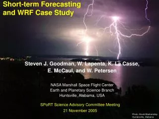
Short-term Forecasting and WRF Case Study Steven J. Goodman W. Lapenta, K. La Casse, E. McCaul, and W. Petersen NASA Marshall Space Flight Center Earth and Planetary Science Branch Huntsville, Alabama, USA. NWS Severe Weather Technology Workshop 12-14 July 2005 Silver Spring, MD.

E N D
Short-term Forecasting and WRF Case Study Steven J. Goodman W. Lapenta, K. La Casse, E. McCaul, and W. Petersen NASA Marshall Space Flight Center Earth and Planetary Science Branch Huntsville, Alabama, USA NWS Severe Weather Technology Workshop 12-14 July 2005 Silver Spring, MD
Outline of Talk • Nowcasting Gaps and Opportunities • WRF-RAMS Case Study- 10 Dec. 2004 • Columbia Project-WRF modeling plans • Concluding Remarks
NWS STIP Solutions (Science and Technology Infusion Plan) Weather Research and Forecast, WRF Data Assimilation, DA Additional Forecast Interests CI- convective initiation TI- first lightning (35 dbZ at -15C) TF- final lightning
*Visionary Forecast and Warning Lead Times *NWS Science and Technology Infusion Plan: Lightning Observation and Forecast Benefit
Nowcasting: forecasting with local detail, by any method, over a period from the present to a few hours ahead; that includes a detailed description of the present weather, and includes the blending of extrapolation, statistical, and heuristic techniques (includes theory, expert systems, fuzzy logic, and forecaster rule of thumb), and NWP Nowcasting Defined
Extrapolation Statistical Model derived forecast fields Convergence line Detection & characterization Radar retrievals Data Fusion System Nowcast NWP Forecast Rules Forecast rules e.q boundary collision storm initiation likely Forecaster Input e.q. convergence line Input, meteorological situation Courtesy, Jim Wilson NCAR WWRP/Tom Keenan
Lightning Connection to Thunderstorm Updraft, Storm Growth and Decay • Total Lightning —responds to updraft velocity and concentration, phase, type of hydrometeors, integrated flux of particles • WX Radar — responds to concentration, size, phase, and type of hydrometeors- integrated over small volumes • Microwave Radiometer — responds to concentration, size, phase, and type of hydrometeors — integrated over depth of storm (85 GHz ice scattering) • VIS / IR — cloud top height/temperature, texture, optical depth
4km horizontal resolution 37 vertical levels Dynamics and physics Eulerian mass core Dudhia SW radiation RRTM LW radiation YSU PBL scheme Noah LSM WSM 6-class microphysics scheme Explicit convection 24h forecast initialized at 00 UTC 10 December 2004 with AWIP212 NCEP EDAS analysis Eta 3-h forecasts used for LBC’s WRF Configuration Cloud cover 18h forecast valid at 18 UTC 10 Dec. 2004
WRF Surface Based CAPE 18h fcst valid 18 UTC Dec 10
MIPS Sounding ~ 761 J/kg CAPE • Low level lapse rates and low freezing level efficient for converting CAPE to kinetic energy • Surface T=15C, Td=10C • Max w= 19 m/s UAH MIPS, Kevin Knupp
WRF 3h Precipitation 18h fcst valid 18 UTC Dec 10
WRF 3h Precipitation 21h fcst valid 21 UTC Dec 10
WRF 3h Precipitation 21h fcst valid 21 UTC Dec 10 Question: Any lightning, when was it, What was WRF reflectivity at -15 C?
WRF Reflectivity (dBZ)18h forecast valid at 18 UTC 10 Dec. 2004 WRF reflectivity cores too shallow -15 C - 0 C - 850 hPa
850 hPa Reflectivity (dBZ)06:50h forecast valid at 18:50 UTC 10 Dec. 2004
Ground-truth Report of Dime-Size Hail Owens Crossroads, Alabama
10 December Hail Case ARMOR collected data! First time ZDR used on television! • Cold upper-low • GOES 2057 J/kg CAPE in a layer about 7.5 km deep • GOES sounding too warm and moist near surface, likely cloud contaminated • Dime to quarter-sized hail reported in SE Madison county and in S. Tennessee
NCAR HYDRO-ID REFLECTIVITY Cloud Drizzle Lt. Rain Mod. Rain Heavy Rain Hail Hail/Rain Small Hail Rain/Sm. Hail Dry Snow Wet Snow Ice Crys. 5 12 20 28 35 43 50 57 HAIL SMALL HAIL RAIN ARMOR 1.3 degree PPI scan at 17:55 UTC on 10 Dec. 04 Particle Identification Reflectivity [dBZ]
Rain/Hail -0.5 to 2 dB ARMOR: 12/10/04 17:55:06 EL=1.3o Rain/Hail 40-55 dBZ dBZ ZDR Hail -1.5 to 0.5 dB Hail 50-55 dBZ Rain 2 to 3.5 dB Rain 55+ dBZ -1.8 -0.9 0.1 1.0 1.9 2.9 3.6 -15 - 5 5 15 25 35 45 Hail 55+ dBZ Hail -1 to 0.5 dB LMA S. Cell 17:52:30 – 17:57:30 At 17:55 IC fl. rate ~ 3/minute in southern cell No IC’s in northern cell at 17:55 No CG’s in either cell for 20 minutes centered on 17:55 Only 3 CG’s detected for duration of storms
RAMS Configuration • 500 m horizontal resolution • Height, Dz is variable, from 250 m at bottom to 750 m at 20 km height • Domain 75 km x 75 km x 24.5 km • Time, Dt = 4 s, five acoustic steps between • Smagorinsky subgrid mixing scheme • 5-class precipitating hydrometeors: • Rain, snow, aggregates, graupel, hail • Initialized with 3K warm bubble, radius=12 km at z=0 • 120 min simulation, initiation effects dominate until t=60 min
RAMS Configuration Graupel • 500 m horizontal resolution • Height, Dz is variable, from 250 m at bottom to 750 m at 20 km height • Domain 75 km x 75 km x 24.5 km • Time, Dt = 4 s, five acoustic steps between • Smagorinsky subgrid mixing scheme • 5-class precipitating hydrometeors: • Rain, snow, aggregates, graupel, hail • Initialized with 3K warm bubble, radius=12 km at z=0 • 120 min simulation, initiation effects dominate until t=60 min
RAMS Configuration Hail • 500 m horizontal resolution • Height, Dz is variable, from 250 m at bottom to 750 m at 20 km height • Domain 75 km x 75 km x 24.5 km • Time, Dt = 4 s, five acoustic steps between • Smagorinsky subgrid mixing scheme • 5-class precipitating hydrometeors: • Rain, snow, aggregates, graupel, hail • Initialized with 3K warm bubble, radius=12 km at z=0 • 120 min simulation, initiation effects dominate until t=60 min
Use of MODIS SST to Improve High Resolution Modeling of Atmosphere/Ocean Interactions within the Gulf of Mexico and Florida Coastal Zones PI: William M. Lapenta/NASA Short-term Prediction Research and Transition Center @ MSFC 100,000 Processor Hours awarded March 2005 Award number: SMD-Dec04- 0036 Objective of Columbia Usage • Enables experimental high-resolution atmospheric modeling at 2 km resolution on an operational basis that would not be possible otherwise • Unique computational resources allows compilation of results for more than a single season • Allows for subjective impact assessment from operational NWS forecast community Identify the codes to be run on Columbia • WRF: Weather Prediction Model • ADAS: Data Assimilation System Sea surface temperature fields (K) mapped to a numerical model 2 km grid near Cape Canaveral, FL. The RTG is a default field used in most models. The MODIS SST composite contains detailed spatial structure that is known to affect weather near and along coastlines associated with mesoscale circulations. Scientific Impact Hypothesis: Accurate specification of the lower-boundary forcing (i.e., the specification of localized SST gradients and anomalies) within the WRF prediction system will result in improved land/sea fluxes and hence, more accurate evolution of coastal mesoscale circulations and the sensible weather elements (i.e., low-level horizontal transport, temperature trends, clouds, and precipitation) associated with them. Key Milestones • Implement and optimize WRF configuration 05/05 • Develop Web-based visualization for model output 05/05 • Conduct simulations on a daily basis 06/05 • Provide output to FL NWSFO’s in AWIPS 07/05 • Preliminary MODIS SST impact assessment 10/05 • Present results at AMS Annual Meeting 01/06 • Prepare manuscript for peer-review publication 03/06 • Report findings to WRF modeling community 03/06 Co-Is/Partners Kate La Casse and Stephanie Haines, University of Alabama in Huntsville Gary Jedlovec, NASA @ MSFC; Scott Dembek (USRA) Steven Lazarus, Florida Institute of Technology Science Mission Directorate - Project Columbia Investigation
cool warm Motivation for using High-Resolution MODIS SST Fields in NWP Models • SST known to influence coastal mesoscale processes • Can impact warm-season precipitation distribution • Sea breeze circulations important to heavily populated areas (HOU, NYC) • Strong influence on height of marine boundary layer
MODIS – RTG (°C) Mapped to MM5 2km grid + 2.0 °C cool warm + 1.5 °C Use of High-Resolution MODIS SST Fields in NWP Models • SST known to influence coastal mesoscale processes • Can impact warm-season precipitation distribution • Sea breeze circulations important to heavily populated areas (HOU, NYC) • Strong influence on height of marine boundary layer