IETF Differentiated Services

1. IETF Differentiated Services Concerns with Intserv: • Scalability: signaling, maintaining per-flow router state difficult with large number of flows • Flexible Service Models: Intserv has only two classes. Also want “qualitative” service classes • “behaves like a wire” • relative service distinction: Platinum, Gold, Silver Diffserv approach: • simple functions in network core, relatively complex functions at edge routers (or hosts) • Do’t define define service classes, provide functional components to build service classes

2. marking r b scheduling . . . Diffserv Architecture Edge router: - per-flow traffic management - marks packets as in-profile and out-profile Core router: - per class traffic management - buffering and scheduling based on marking at edge - preference given to in-profile packets - Assured Forwarding

3. Rate A B Edge-router Packet Marking • profile: pre-negotiatedrate A, bucket size B • packet marking at edge based on per-flow profile User packets Possible usage of marking: • class-based marking: packets of different classes marked differently • intra-class marking: conforming portion of flow marked differently than non-conforming one

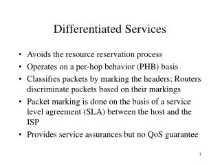
4. Classification and Conditioning • Packet is marked in the Type of Service (TOS) in IPv4, and Traffic Class in IPv6 • 6 bits used for Differentiated Service Code Point (DSCP) and determine PHB that the packet will receive • 2 bits are currently unused

5. Classification and Conditioning may be desirable to limit traffic injection rate of some class: • user declares traffic profile (eg, rate, burst size) • traffic metered, shaped if non-conforming

6. Forwarding (PHB) • PHB result in a different observable (measurable) forwarding performance behavior • PHB does not specify what mechanisms to use to ensure required PHB performance behavior • Examples: • Class A gets x% of outgoing link bandwidth over time intervals of a specified length • Class A packets leave first before packets from class B

7. Forwarding (PHB) PHBs being developed: • Expedited Forwarding: pkt departure rate of a class equals or exceeds specified rate • logical link with a minimum guaranteed rate • Assured Forwarding: 4 classes of traffic • each guaranteed minimum amount of bandwidth • each with three drop preference partitions

8. Diffserv and MPLS • Both are WAN QoS mechanisms. While Diffserv is used for traffic aggregation and provisioning of differentiated services, MPLS is mainly used for traffic aggregation and load balancing.

9. MPLS • Originally introduced as a WAN mechanism for forwarding packets using label switching instead of the IP address-based routing and provide differentiated QoS. • It has found its most use in Traffic Engineering (TE) • TE requires that traffic follows specific, possibly nonoptimal, routes to enable diverse routing, traffic load balancing, and other means of optimizing network resources. • MPLS forces traffic into these routes or Label Switched Paths (LSPs).

10. Routers or LSRs • In the MPLS network, routers are called label switching routers (LSR). • Edge LSRs (also called LERs) provide the interface between the external IP network and the LSP. • Core LSRs provide transit services through the MPLS cloud using the pre-established LSP. • In a SP network, on the ingress the Edge LSR accepts IP packets and appends MPLS labels. • On the egress, an edge LSR terminates the LSP by removing MPLS labels and resorting to the normal IP forwarding.

11. FEC • The forward equivalence class (FEC) is a representation of a group of packets that share the same requirements for their transport. All packets in such a group are provided the same treatment en route to the destination. • Each LSR builds a table to specify how a packet must be forwarded. The table, label information base (LIB) comprises of FEC-to-label bindings.

12. Labels and Label Bindings • A label identifies the path a packet should traverse • It is encapsulated in a layer-2 header of the packet -- special MPLS header (aka shim) includes a label, an experimental field (Exp), an indicator of additional labels(S), and Time to live (TTL). • Receiving router uses the label content to determine the next hop. • Label values are of local significance only pertaining to hops between LSRs. • Labels are bound to an FEC asa result of some event or policy

13. Label Assignment • Based on forwarding criteria such as • destination unicast routing • traffic engineering • multicast • virtual private network • QoS

14. MPLS Signaling • A signaling protocol performs a variety of functions such as: • setting up LSPs traversing specified sequences of LSRs derived from the constraint-based routing (CR) analysis; • create the path state in each LSR by performing label allocation, distribution, and binding; • reserve resources in each LSR including bandwidth, delay, and packet loss bounds; • eassign the network resources as necessary; • dynamically reroute during network congestion and failures; • monitor and maintain explicitly routed LSP state

15. CR-LDP • CR-LDP: LDP using constraint-based routing • LDP provides a common understanding between LSR peers of the meaning of labels used to forward traffic between them • Message categories: • Discovery -- sent periodically by LSRs to announce their presence • Session -- to establish, maintain, and terminate a session between two LDP peers • Advertisement -- to create, change, and delete label mappings to FECs after a session has been established • Notification -- to signal and provide advisory info. • Forward path, hard state with no state refreshes

16. RSVP-TE • Signals between LSRs • Creates a state for a collection of flows between the ingress and egress points of a traffic trunk • An LSP aggregates multiple host-to-host flows and thus reduces the amount of RSVP states in the network • Uses firm state where Path and Resv messages are periodically refreshed but their volume is significantly reduced

17. QoS Routing • As defined in RFC 2386, QoS “is a set of service requirements to be met by the network while transporting a flow.” A flow is “a packet stream from source to a destination with an associated QoS.” • Measurable level of service delivered to network users which can be characterized by packet loss probability, available bandwidth, end-to-end delay, etc. Expressed as a Service Level Agreement(SLA) between network users and service providers. • QoS-based routing is defined as “a routing mechanism under which paths for flows are determined based on some knowledge of resource availability in the network as well as the QoS requirement of the flows.” A dynamic routing scheme with QoS considerations.

18. QoS Metrics • Bandwidth, delay, jitter, cost, loss probability • three types of metrics: additive, multiplicative, concave • Let m(n1,n2) be a metric for link(n1, n2). For any path P = (n1, n2, .., ni, nj), metrci m is: • additive, if m(P) = m(n1,n2) + m(n2,n3) +…..+ m(ni,nj) (examples are dealy, jitter, cost, hop-count) • multiplicative, if m(P) = m(n1,n2) * m(n2,n3) *…* m(ni,nj) (example is reliability, in which case 0<=m(ni,nj)<=1) • concave, if m(P) = min{m(n1,n2), m(n2,n3), …, m(ni,nj)} (example is bandwidth meaning that the bandwidth of the path as a whole is determined by the link with the minimum available bandwidth)

19. Objectives • To meet QoS requirements of end users. • To optimize network resource usage • to gracefully degrade network performance under heavy load

20. Design Issues(1) • IP routing protocols such as OSPF, RIP, and BGP are called “best-effort” routing protocols. They use only the shortest path to the destination -- single objective optimization algorithms which consider only one metric (like hop-count). • Much more difficult to design and implement than Best-effort routing. Many tradeoffs have to be made. In most cases the goal is not to find the best solution but to find a viable solution with acceptable cost.

21. Design Issues(2) • Metrics and path computation • how do we measure and collect network state information? • how do we compute routes based on the information collected? • Mapping of QoS requirements to well defined QoS Metrics • Computation complexity associated with path computation (much of QoS routing based on multiple constraint optimization is NP-complete). Many heuristic algorithms exist.

22. Design Issues (3) • Path computation is followed by resource reservation which means that when the path is chosen the network state in terms of available resources is changed and such information needs to propagated throughout the network. • Knowledge propagation and Maintenance • how often the routing information is exchanged between the routers? • The tradeoff here is between information accuracy and efficiency. • For instance, what is available bandwidth? Is it what is left after reservation or the actual physically available? • How do we maintain the info collected?(on demand path computation, aggregation, routing tables?)

23. Design Issues (4) • Scaling by hierarchical aggregation • Imprecise state information model. Sources of inaccuracy: • network dynamics • aggregation of routing information • hidden information • approximate calculation • Administrative control -- flow priorities and preemption, resource control and fairness • Integrate QoS-based routing and Best-effort routing

24. Intra-domain Vs. Inter-domain • Dynamic path computation to statically provisioned paths for a few service classes for intra-domain • Some common features for intra-domain: • admission control, optimal resource usage, failure notices, support for best-effort flows, support for multicast routing with receiver heterogeneity and shared reservation styles • Inter-domain routing scheme have to be scalable and therefore, simple. • Cannot be based on highly dynamic network state info • info exchange between domains should be relatively static

25. Routing Strategies • Source routing • distributed routing • hierarchical routing • they are classified based on the way the state information is maintained and the search foe feasible path is carried out

26. Source Routing • Each node maintains the complete global state, including the network topology and the state information of every link • Based on the global state, a feasible path is locally computed at the source node • A control message is sent out along the selected path to inform the intermediate nodes of their precedent and successive nodes • A link state protocol is used to update the global state at every node

27. Source Routing (2) • Strengths: simplicity through centralization; avoids many of the distributed computing problems; guarantees loop-free routes; conceptually simple, easy to implement, evaluate, debug and upgrade; centralized heuristics are much easier to design for some NP-complete routing problems. • Weaknesses: communication overhead to maintain global state; imprecision global state info; high computation overhead at the source; In short, source routing has scalability problem.

28. Distributed Routing • Path is computed by a distributed computation • Control messages are exchanged among nodes and state information kept at each node is collectively used for path search • Requires a distance-vector protocol or link-state protocol to maintain a global state in the form of distance vectors at every node. Based on the distance vectors, the routing is done on a hop-by-hop basis.

29. Distributed Routing (2) • Strengths: path computation is distributed and result in shorter routing response time; scalable; searching multiple paths in parallel for a feasible path; routing decision and optimization is done entirely based on local states; • Weaknesses: dependence on global state; flooding based algorithms which do not maintain global state have higher communication overheads; difficult to design efficient heuristics in the absence of detailed topology or link-state info; presence of loops due to inaccurate global state info at individual nodes (easily detected but alternate paths are difficult to find)

30. Hierarchical Routing • Nodes are clustered into groups which may be clustered into higher level groups recursively creating a multi-level hierarchy. • Each physical node maintains an aggregated global state -- contains the detailed state info about the nodes in the same group and aggregated state info about other groups. • Source routing is used to find a feasible path. • A control message is sent along this path to establish the connection. A border node in a group represented by a logical node receives the message and uses source routing to extend the path through the group.

31. Hierarchical Routing (2) • Strengths: Scales well; retains many advantages of source routing as well as distributed routing. • Weaknesses: aggregated network state introduces additional imprecision; gets more complicated when multiple QoS constraints are involved.

32. QoS Routing Algorithms • For Unicast, the problem is to find a network Path that meets the requirement of a connection between two end users • For multicast, the problem is to find a multicast tree rooted at the sender and the tree covers all receivers with every internal path from the sender to a receiver satisfying the requirement • QoS requirement as a set of constraints • link constraint (concave metrics) • path constraint (additive and multiplicative metrics) • tree constraint

33. Algorithms • Feasible path is one that has sufficient residual resources to satisfy the QoS constraints of a connection • In addition to a feasible path, we also want to optimize resource utilization -- measured by an abstract metric cost • Cost could be in dollars or a function of the buffer or b/w utilization. Cost of a path is the total cost of all links on the path • the optimization problem is to find the least-cost path among all feasible paths.

34. Difficulties • Diverse applications and different QoS requirements. Multiple constraints often make the routing problem intractable -- finding a path with two independent path constraints is NP-complete. • Difficult to determine the optimal operating point for both QoS and Best effort traffic if their distributions are different. Best-effort traffic will suffer if overall traffic distribution is misjudged • Maintaining up-to-date network state as it changes dynamically due to transient load fluctuation, connections in and out and links up and down.

35. Graph-based Models • A network modeled as a graph <V, E>. Nodes (V) represent switches, routers, and hosts. Edges (E) represent communication links. Symmetric or asymmetric links. • Link state may be a triple consisting of residual b/w, delay, cost • Node state can be combined into the state of the adjacent links • The delay of a link consists of the link propagation delay and queueing delay at the node. The cost of alink is determined by the total resource consumption at the link and the node.

36. State Information • Local state: each node is assumed to maintain its up-to-date local state including all delays, residual b/w on the outgoing links, and the availability of other resources • Global state: The combination of the local states of all nodes. Every node is able to maintain the global state by either a link-state protocol or a distance-vector protocol which exchanges the local states among the nodes periodically. • Link state protocols broadcast the local state of every node to every other node. Distance vector protocols periodically exchange distance vectors among adjacent nodes. Figures 1 and 2

37. Aggregate global state • Figure 3

38. Links and paths • For some metrics, the state of a path is determined by the state of the bottleneck link • link optimization routing -- find a path that has the largest bandwidth on the bottleneck link -- widest path • link-constrained routing -- find a path whose bottle neck bandwidth is above a required value (reduced to link optimization problem after pruning) • for some other metrics, the state of the path is determined by the combined state over all links on the path • path optimization -- least cost routing • path constrained -- delay constrained

39. NP-Complete problem classes • PCPO -- delay-constrained least-cost routing find the least cost path with bonded delay • MPC -- delay-delayjitter constrained routing find a path with both bounded delay and bounded delay jitter • These two classes are NP-complete if the QoS metrics are independent and if they are allowed to be real numbers or unbounded integer numbers. • Solvable in polynomial time if all but one metric take bounded integers; Also if all metrics are dependent on a common metric (ex. worst-case delay and delay jitter are functions of b/w in WFQ)

40. Chen-Nahrstedt • Heuristic for multi-path constrained routing problem. Example: delay-cost constrained • map the cost (or delay) of every link from an unbounded real number to a bounded integer; Solvable in polynomial time

41. Source Routing Algorithms • Maintain a global state at every node • most algorithms transform the routing problem to a shortest path problem and then solve it by Dijkstra’s or Bellman-Ford algorithm.

42. Salama et. al. Algorithm • Distributed heuristic algorithm for delay-constrained least cost routing problem. • A cost vector and a delay vector are maintained at every node by a distance vector protocol • The cost(delay) vector contains for every destination the next node on the least-cost (least-delay) path. • A control message is sent from the source toward the destination to construct a delay-constrained path. Loops may occur and detected if the control message visits a node twice. Routing process is rolled back until reaching a node from which the least-cost path was followed.

43. Sun-Landgendorfer • Improves worst-case performance of Salama et. al. by avoiding loops instead of detecting and removing loops. • A control message is sent to construct the path • The message travels along the least-delay path until reaching a node from which the delay of the least-cost path violates the delay constraint.

44. PNNI and QOSPF • Hierarchical link-state routing protocol • Topology information is flooded through the network -- change (LSA)propagated based on a threshold model • Traffic classes may be defined to indicate network resource requirements • Widest-shortest path (which is a minimum hop count path with maximum bandwidth) may be pre-computed for every possible destination.