Download
1 / 44
450 likes | 588 Vues
Clause Learning in a SAT -Solver. „Those who do not learn from their mistakes are doomed to repeat them “. Presented by Richard Tichy and Thomas Glase. Introduction. Motivation Definitions Conflict-Clause I-Graph Cuts Decision levels Learning schemes (1UIP, Rel_Sat, GRASP…)

E N D
Clause Learning inaSAT-Solver „Those who do not learn from their mistakes are doomed to repeat them“ Presented by Richard Tichy and Thomas Glase
Introduction • Motivation • Definitions • Conflict-Clause • I-Graph • Cuts • Decision levels • Learning schemes (1UIP, Rel_Sat, GRASP…) • Conflict clause maintenance • Bounded learning • Efficient data structures • Clause learning and restarts • Complexity • Benchmark results and comparison • Conclusion
Motivation • Naive backtracking schemes jump back to the most recent choice variable assigned. • Possibility exists of recreating sub trees involving conflicts. • Performance can be improved by using backjumping(with learning). • Backjumping (with learning) improves on naive backtracking. • Prunes previously discovered sections of the search tree that can never contain a solution.
DPLL algorithm (recursive) procedure DPLL(П,α) execute UP on (П,α); if empty clause in П then return UNSATISFIABLE; ifП is total then exit with SATISFIABLE; choose a decision literal p occurring in П\α; DPLL(П U {(p)}, α U {p}); DPLL(П U {(¬p)}, α U {¬p}); return UNSATISFIABLE;
Conflict Directed Clause Learning (CDCL) procedure CDCL( П ) Γ = П, α= Ø, level = 0 repeat: execute UP on (Γ, α) if a conflict was reached iflevel = 0 return UNSATISFIABLE C = the derived conflict clause p = the sole literal of C set at the conflict level level = max{ level(x) : x is an element of C – p} α = αless all assignments made at levels greater than level (Γ, α) = (ΓU {C}, αp) else if αis total return SATISFIABLE choose a decision literal p occurring in Γ\α α = αp increment level end if
A Small Example • literals numbered x1 to x9 • formula consists of clauses 1 to 6: 1 = (x1 x2) 2 = (x1 x3 x7) 3 = (x2 x3 x4) 4 = (x4 x5 x8) 5 = (x4 x6 x9) 6 = (x5 x6) Start by choosing literal x7 with assignment 0 (decision level 1)
x8 = 0@2 UP = Ø x9 = 0@3 UP = Ø x1= 0@4 UP = {x2=1, x3=1, x4=1, x5=1, x6=1, x5=0} Propagation adds nothing at decision levels 1, 2 and 3. Propagation at level 4 leads to conflicting literal assignments. Motivation 1 = (x1 x2) 2 = (x1 x3 x7) 3 = (x2 x3 x4) 4 = (x4 x5 x8) 5 = (x4 x6 x9) 6 = (x5 x6) x7= 0@1 UP = Ø
Background (Learning in SAT) • Learning involves generating and recording conflict clauses discovered during unit propagation. • Generating conflict clauses involves analyzing the implication graph (i-graph) at the time of a conflict. • Different learning schemes correspond to different cuts in the i-graph. • Cuts are used to generate conflict clauses and provide a backtracking level. • Some definitions are needed to further understand the implication graph and a cut.
Motivation • Definitions • Conflict-Clause • I-Graph • Cuts • Decision levels • Learning schemes (1UIP, Rel_Sat, GRASP…) • Conflict clause maintenance • Bounded learning • Efficient data structures • Clause learning and restarts • Complexity • Benchmark results and comparison • Conclusion
Definitions: Conflict clause • A conflict clause represents an assignment to a subset of the variables from the problem that can never be part of a solution. • Learning in SAT involves finding and recording these conflict clauses (in CSP and ASP as well). • Contributes heavily to the success of the best SAT and CSP solvers, only recently attempted with ASP problems.
Definitions: Conflict clauses cont. • Properties: • Asserting clause • Contains exactly one literal assigned at conflict level • Logically implied by original set of formula (correctness) • Must be made false by variable assignment involving the conflict
Definitions: Implication graph Implication graph: A directed acyclic graph where each vertex represents a variable assignment (e.g. a literal in SAT). • An incident edge to a vertex represents the reason leading to that assignment. • Decision variables have no incident edges. • Implied variables have assignments forced during UP. • Each variable (decision or implied) within the implication graph has a decision level associated with it. • If the graph contains a variable assigned both 1 and 0 (x and ¬x both exist in the graph) than the implication graph contains a conflict.
Definitions: Implication graph Building the i-graph: • Add a node for each decision labelled with the literal (no incident edges). • While there exists a known clause C=(l1 v… lk v l ) such that ¬l1 ,… ,¬lk are in G. • Add a node labeled l if not already in G. • Add edges (li ,l ) for 1 ≤ i ≤ k if not already extant in G. • Add C to the label set of these edges to associate the edges as a group with clause C. • (optional) Add a node λ to the graph and add a directed edge from the variable occurring both positively and negatively to λ.
4 x2=1@4 x5=1@4 1 4 3 x4=1@4 x5=0@4 6 3 2 5 2 5 x6=1@4 x3=1@4 Definitions: Implication graph Current partial assignment: { x7=0@1 ,x8=0@2, x9=0@3} Current decision assignment: {x1=0@4} x8=0@2 1 = (x1 x2) 2 = (x1 x3 x7) 3 = (x2 x3 x4) 4 = (x4 x5 x8) 5 = (x4 x6 x9) 6 = (x5 x6) x1=0@4 x9=0@3 x7=0@1
More Definitions… Conflict Side: The i-graph bipartition, or cut, containing the conflicting nodes Reason Side: The nodes of the i-graph bipartition not included in the conflict side. Unique Implication Point (UIP): Any node at the current decision level such that any path from the decision variable to the conflict variable must pass through it.
Learning Schemes • Different SAT learning schemes correspond to different cuts in the graph. • Intuitively, different cuts correspond to different extensions of the conflict side of the i-graph. • Different cuts generate different conflict clauses. • These conflict clauses are added to the database of clauses. • This storage of clauses represents the learned portion of the search.
Learning Schemes • 1 UIP (MiniSAT, zChaff) • Rel_Sat • GRASP • Etc…
4 x2=1@4 x5=1@4 1 4 3 x4=1@4 x5=0@4 6 3 2 5 2 5 x6=1@4 x3=1@4 Learning Schemes (1 UIP) Reason Side x8=0@2 1 = (x1 x2) 2 = (x1 x3 x7) 3 = (x2 x3 x4) 4 = (x4 x5 x8) 5 = (x4 x6 x9) 6 = (x5 x6) Conflict Side x1=0@4 x9=0@3 x7=0@1
1 UIP Cut 4 x2=1@4 x5=1@4 1 4 3 x4=1@4 x5=0@4 6 3 2 5 2 5 x6=1@4 x3=1@4 Learning Schemes (1 UIP) Reason Side x8=0@2 1 = (x1 x2) 2 = (x1 x3 x7) 3 = (x2 x3 x4) 4 = (x4 x5 x8) 5 = (x4 x6 x9) 6 = (x5 x6) Conflict Side x1=0@4 x9=0@3 x7=0@1
1 UIP Cut 4 x2=1@4 x5=1@4 1 4 3 x4=1@4 x5=0@4 6 3 2 5 2 5 x6=1@4 x3=1@4 Learning Schemes (1 UIP) Reason Side x8=0@2 1 = (x1 x2) 2 = (x1 x3 x7) 3 = (x2 x3 x4) 4 = (x4 x5 x8) 5 = (x4 x6 x9) 6 = (x5 x6) Conflict Side x1=0@4 x9=0@3 x7=0@1 Conflict Clause: C = (x4 x8 x9)
x8 = 0@2 UP = Ø x9 = 0@3 UP = Ø x1= 0@4 UP = {x2=1, x3=1, x4=1, x5=1, x6=1, x5=0} Effect on Backtracking 1 = (x1 x2) 2 = (x1 x3 x7) 3 = (x2 x3 x4) 4 = (x4 x5 x8) 5 = (x4 x6 x9) 6 = (x5 x6) C = (x4 x8 x9) x7 = 0@1 UP = Ø Backtrack to level = max{ level(x) : x is an element of C – p} p = x4 level = 3
x8 = 0@2 UP = Ø x9 = 1@3 Effect on Backtracking 1 = (x1 x2) 2 = (x1 x3 x7) 3 = (x2 x3 x4) 4 = (x4 x5 x8) 5 = (x4 x6 x9) 6 = (x5 x6) C = (x4 x8 x9) x7 = 0@1 UP = Ø … Current partial assignment: {x7=0, x8=0, x9=1, x4=1}
4 x2=1@4 x5=1@4 1 4 3 x4=1@4 x5=0@4 6 3 2 5 2 5 x6=1@4 x3=1@4 Learning Schemes (Rel_Sat) Reason Side x8=0@2 1 = (x1 x2) 2 = (x1 x3 x7) 3 = (x2 x3 x4) 4 = (x4 x5 x8) 5 = (x4 x6 x9) 6 = (x5 x6) Conflict Side x1=0@4 x9=0@3 x7=0@1
Last UIP Cut 4 x2=1@4 x5=1@4 1 4 3 x4=1@4 x5=0@4 6 3 2 5 2 5 x6=1@4 x3=1@4 Learning Schemes (Rel_Sat) Reason Side x8=0@2 1 = (x1 x2) 2 = (x1 x3 x7) 3 = (x2 x3 x4) 4 = (x4 x5 x8) 5 = (x4 x6 x9) 6 = (x5 x6) Conflict Side x1=0@4 x9=0@3 x7=0@1
4 x2=1@4 x5=1@4 1 4 3 x4=1@4 x5=0@4 6 3 2 5 2 5 x6=1@4 x3=1@4 Learning Schemes (Rel_Sat) Reason Side Last UIP Cut x8=0@2 1 = (x1 x2) 2 = (x1 x3 x7) 3 = (x2 x3 x4) 4 = (x4 x5 x8) 5 = (x4 x6 x9) 6 = (x5 x6) Conflict Side x1=0@4 x9=0@3 x7=0@1 Conflict Clause: C = (x1 x7 x8 x9)
4 x2=1@4 x5=1@4 1 4 3 x4=1@4 x5=0@4 6 3 2 5 2 5 x6=1@4 x3=1@4 Learning Schemes (GRASP) Reason Side x8=0@2 1 = (x1 x2) 2 = (x1 x3 x7) 3 = (x2 x3 x4) 4 = (x4 x5 x8) 5 = (x4 x6 x9) 6 = (x5 x6) Conflict Side x1=0@4 x9=0@3 x7=0@1
1 UIP Cut 4 x2=1@4 x5=1@4 1 4 3 x4=1@4 x5=0@4 6 3 2 5 2 5 x6=1@4 x3=1@4 Learning Schemes (GRASP) Reason Side x8=0@2 1 = (x1 x2) 2 = (x1 x3 x7) 3 = (x2 x3 x4) 4 = (x4 x5 x8) 5 = (x4 x6 x9) 6 = (x5 x6) Conflict Side x1=0@4 x9=0@3 x7=0@1
1 UIP Cut 4 x2=1@4 x5=1@4 1 4 3 x4=1@4 x5=0@4 6 3 2 5 2 5 x6=1@4 x3=1@4 Learning Schemes (GRASP) Reason Side x8=0@2 1 = (x1 x2) 2 = (x1 x3 x7) 3 = (x2 x3 x4) 4 = (x4 x5 x8) 5 = (x4 x6 x9) 6 = (x5 x6) Conflict Side x1=0@4 x9=0@3 x7=0@1 Conflict Clause: C = (x4 x8 x9) ( Flip Mode ) Additional Clause: C1 = (x1 x7 x4)
1 UIP Cut 4 x2=1@4 x5=1@4 1 4 3 x4=1@4 x5=0@4 6 3 2 5 2 5 x6=1@4 x3=1@4 Learning Schemes (GRASP) Reason Side x8=0@2 1 = (x1 x2) 2 = (x1 x3 x7) 3 = (x2 x3 x4) 4 = (x4 x5 x8) 5 = (x4 x6 x9) 6 = (x5 x6) C = (x4 x8 x9) C1 = (x1 x7 x4) Conflict Side x1=0@4 x9=0@3 x7=0@1 Conflict Clause: C2 = (x7 x8 x9) ( Backtracking Mode )
Motivation • Definitions • Conflict-Clause • I-Graph • Cuts • Decision levels • Learning schemes (1UIP, Rel_Sat, GRASP…) • Conflict clause maintenance • Bounded learning • Efficient data structures • Clause learning and restarts • Complexity • Benchmark results and comparison • Conclusion
Conflict Clause Maintenance • Every conflict can potentially add conflict clauses to the database. • Conflict clauses can become large as the search progresses. • Unrestricted learning can add a prohibitive overhead in terms of space. • Time in UP increases with number of learned clauses added. • Retaining all learned clauses is impractical. • Strategies exist to help alleviate these problems.
Conflict Clause Maintenance Consider conflict clause (x1 x7 x8 x9) (added by rel_sat) Consider α = {x7=0, x2=1, x4=0, x6=1, x5=0} • clause would be deleted using relevance bounding when i ≥ 3 • clause would be deleted using size-bounded learning when e.g. i ≥ 4
Conflict Clause Maintenance • Relevance-bounded and Size-bounded learning can alleviate some of the space problems of unrestricted learning [3]. • Relevance Bounded Learning: Maintains conflict clauses that are considered more relevant to the current search space. • i-relevance means that a reason is no longer relevant when > i literals in the clause are currently unassigned. • Size-Bounded Learning: Maintains only those clauses containing ≤ i variables. • Periodically remove clauses from database based on one (or a combination) of the above strategies.
Efficient Data Structures Efficient data structures can reduce memory ‘footprint’. • Cache aware implementations try to avoid cache misses: • by using arrays rather than pointer based data structures. • by storing data in such a way that memory accesses involve contiguous memory locations. • Special data structures for short clauses: • keep a list for each literal p of all literals q for which there is a binary clause (¬p v q) . • scan list when assigning p true. • can be extended to ternary clauses. • Clause ordering by size during UP. • Watched literals rather than counters. All of the above reduce UP time and conserve memory.
Clause Learning and Restarts • Search may enter area where useful conflict clauses are not produced. • Restarts throw away the current literal assignment (except initial UP) and start search again. • Retains cache of the learned clauses from the previous start and this usually results in a different search. • learned clauses typically larger than input formula • learned clauses affect choice of decision variables • choice of decision variable affects search path
Clause Learning and Restarts • Restarts sacrifice completeness: • Unless all learned clauses are maintained for all restarts the search space may never be completely examined. • Maintaining all learned clauses not feasible. • Some solvers maintain completeness by gradually increasing interval for restarts to ∞.
Complexity • Learning Schemes implemented by Implication Graph Traversal • Time Complexity: O(V+E)
Benchmark Results and Comparison • Comparing fixed branching to VSIDS heuristic • Fixed heuristic branches on unassigned variable with smallest index (variables preordered) • VSIDS – Variable State Independent Decaying Sum • for each literal ℓ in the formula keep a score s(ℓ) which is initially the number of occurrences in the formula • increment s(ℓ) each time a clause with ℓ is added • after N decisions recompute all s(ℓ) = r(ℓ) + s(ℓ)/2 • r(ℓ) = number of occurrences of ℓ in conflict clauses since last update. • choose ℓ with highest s(ℓ)
Benchmark Results and Comparision • Results clearly show that while VSIDS decision heuristic may not always be faster, it is certainly more robust. • 1UIP outperformed rel_sat and GRASP in all but 2 benchmarks. • SAT-Competition Winner 2005 (Industrial Cases): SATElite based on MiniSAT incorporates 1UIP learning scheme and VSIDS decision heuristic
Conclusion • Learning potentially speeds up solving process by pruning the search space. • Reasons for conflicts are recorded to avoid the same mistakes in the future. • Conflict clause maintenance necessary for practical applications. • Bounded Learning and efficient data structures reduce memory footprint and speed up UP. • Clause learning adds power to restart strategy. • 1UIP outperforms all other learning schemes in most benchmarks. • Clause learning is a major step in the efficiency of SAT-Solvers.
References • [1] Bayardo, R. and Shrag, R. Using CSP Look-Back Techniques to Solve Real-World SAT Instances. Proc. of the Int’l Conf. on Automate Deduction, 1997. • [2] Paul Beame, Henry A. Kautz, Ashish Sabharwal. Understanding the Power of Clause Learning. IJCAI, 2003, 1194-1201.[3] Rina Dechter and Daniel Frost. Backjump-based backtracking for constraint satisfaction problems. Artificial Intelligence, 136(2). 2002, 147--188. • [3] David G. Mitchell, A SAT Solver Primer • [4] Lifschitz, V. Foundations of logic programming. In Brewka, G., ed., Principles of Knowledge Representation. CSLI Publications. 1996., 69-128. • [5] Marques-Silva, J.P. and K.A. Sakallah. GRASP: A Search Algorithm for Propositional Satisfiability. IEEE Trans. on Computers 48(5), 1999, 506-521. • [6] M. Moskewicz, C. Madigan, Y. Zhao, L. Zhang, and S. Malik, CHAFF: Engineering an efficient SAT solver. Proc. Design Automation Conf., 2001, 530-535.
References cont. • [7] L. Zhang, C. F. Madigan, M. H. Moskewicz and S. Malik, Efficient Conflict Driven Learning in a Boolean Satisfiability Solver, Proc. ICCAD, 2001, 279-285. • [8] http://iew3.technion.ac.il/~ofers/courses/advanced/advanced_7.ppt#28