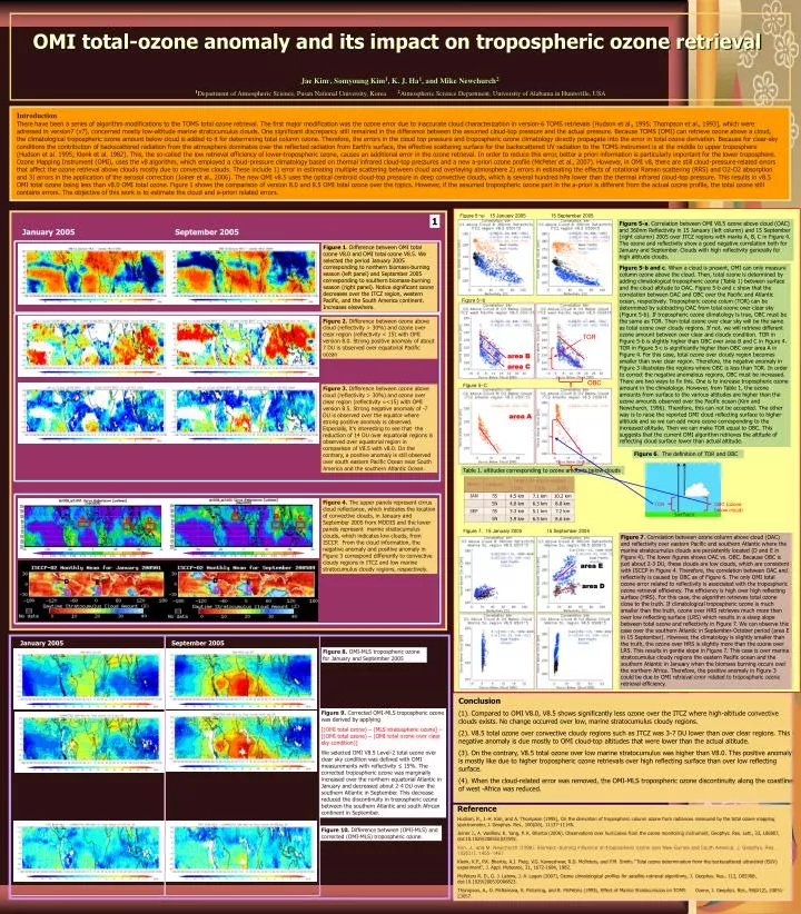
OMI total-ozone anomaly and its impact on tropospheric ozone retrieval

1. OMI total-ozone anomaly and its impact on tropospheric ozone retrieval Jae Kim1, Somyoung Kim1, K. J. Ha1, and Mike Newchurch2 1Department of Atmospheric Science, Pusan National University, Korea 2Atmospheric Science Department, University of Alabama in Huntsville, USA Introduction There have been a series of algorithm modifications to the TOMS total ozone retrieval. The first major modification was the ozone error due to inaccurate cloud characterization in version-6 TOMS retrievals [Hudson et al., 1995; Thompson et al., 1993], which were adressed in version7 (v7), concerned mostly low-altitude marine stratocumulus clouds. One significant discrepancy still remained in the difference between the assumed cloud-top pressure and the actual pressure. Because TOMS (OMI) can retrieve ozone above a cloud, the climatological tropospheric ozone amount below cloud is added to it for determining total column ozone. Therefore, the errors in the cloud top pressure and tropospheric ozone climatology directly propagate into the error in total ozone derivation. Because for clear-sky conditions the contribution of backscattered radiation from the atmosphere dominates over the reflected radiation from Earth’s surface, the effective scattering surface for the backscattered UV radiation to the TOMS instrument is at the middle to upper troposphere (Hudson et al. 1995; Klenk et al. 1982). This, the so-called the low retrieval efficiency of lower-tropospheric ozone, causes an additional error in the ozone retrieval. In order to reduce this error, better a priori information is particularly important for the lower troposphere. Ozone Mapping Instrument (OMI), uses the v8 algorithm, which employed a cloud-pressure climatology based on thermal infrared cloud-top pressures and a new a-priori ozone profile (McPeter et al., 2007). However, in OMI v8, there are still cloud-pressure-related errors that affect the ozone retrieval above clouds mostly due to convective clouds. These include 1) error in estimating multiple scattering between cloud and overlaying atmosphere 2) errors in estimating the effects of rotational Raman scattering (RRS) and O2-O2 absorption and 3) errors in the application of the aerosol correction (Joiner et al., 2006). The new OMI v8.5 uses the optical centroid cloud-top pressure in deep convective clouds, which is several hundred hPa lower than the thermal infrared cloud-top pressure. This results in v8.5 OMI total ozone being less than v8.0 OMI total ozone. Figure 1 shows the comparison of version 8.0 and 8.5 OMI total ozone over the topics. However, if the assumed tropospheric ozone part in the a-priori is different from the actual ozone profile, the total ozone still contains errors. The objective of this work is to estimate the cloud and a-priori related errors. Figure 5-a: 15 January 2005 15 September 2005 1 Figure 5-a. Correlation between OMI V8.5 ozone above cloud (OAC) and 360nm Reflectivity in 15 January (left column) and 15 September (right column) 2005 over ITCZ regions with marks A, B, C in Figure 4. The ozone and reflectivity show a good negative correlation both for January and September. Clouds with high reflectivity generally for high altitude clouds. January 2005 September 2005 Figure 1. Difference between OMI total ozone V8.0 and OMI total ozone V8.5. We selected the period January 2005 corresponding to northern biomass-burning season (left panel) and September 2005 corresponding to southern biomass-burning season (right panel). Notice significant ozone decreases over the ITCZ region, western Pacific, and the South America continent. Increases elsewhere. Figure 5-b and c. When a cloud is present, OMI can only measure column ozone above the cloud. Then, total ozone is determined by adding climatological tropospheric ozone (Table 1) between surface and the cloud altitude to OAC. Figure 5-b and c show that the correlation between OAC and OBC over the Pacific and Atlantic ocean, respectively. Tropospheric ozone colum (TOR) can be determined by subtracting OAC from total ozone over clear sky (Figure 5-b). If tropospheric ozone climatology is true, OBC must be the same as TOR. Then total ozone over clear sky will be the same as total ozone over cloudy regions. If not, we will retrieve different ozone amount between over clear and cloudy condition. TOR in Figure 5-b is slightly higher than OBC over area B and C in Figure 4. TOR in Figure 5-c is significantly higher than OBC over area A in Figure 4. For this case, total ozone over cloudy region becomes smaller than over clear region. Therefore, the negative anomaly in Figure 3 illustrates the regions where OBC is less than TOR. In order to correct the negative anomalous regions, OBC must be increased. There are two ways to fix this. One is to increase tropospheric ozone amount in the climatology. However, from Table 1, the ozone amounts from surface to the various altitudes are higher than the ozone amounts observed over the Pacific ocean (Kim and Newchurch, 1996). Therefore, this can not be accepted. The other way is to raise the reported OMI cloud reflecting surface to higher altitude and so we can add more ozone corresponding to the increased altitude. Then we can make TOR equal to OBC. This suggests that the current OMI algorithm retrieves the altitude of reflecting cloud surface lower than actual altitude. Figure 5-b Figure 2. Difference between ozone above cloud (reflectivity > 30%) and ozone over clear region (reflectivity < 15) with OMI version 8.0. Strong positive anomaly of about 7 DU is observed over equatorial Pacific ocean TOR area B area C OBC Figure 5-C Figure 3. Difference between ozone above cloud (reflectivity > 30%) and ozone over clear region (reflectivity =<15) with OMI version 8.5. Strong negative anomaly of -7 DU is observed over the equator where strong positive anomaly is observed. Especially, it’s interesting to see that the reduction of 14 DU over equatorial regions is observed over equatorial region in comparison of V8.5 with v8.0. On the contrary, a positive anomaly is still observed over south eastern Pacific Ocean near South America and the southern Atlantic Ocean. area A Figure 6. The definition of TOR and OBC Table 1. altitudes corresponding to ozone amounts below clouds Figure 4. The upper panels represent cirrus cloud reflectance, which indicates the location of convective clouds, in January and September 2005 from MODIS and the lower panels represent marine stratocumulus clouds, which indicates low clouds, from ISCCP. From the cloud information, the negative anomaly and positive anomaly in Figure 3 correspond differently to convective cloudy regions in ITCZ and low marine stratocumulus cloudy regions, respectively. A B C A B C Figure 7. 15 January 2005 15 September 2005 Figure 7. Correlation between ozone column above cloud (OAC) and reflectivity over eastern Pacific and southern Atlantic where the marine stratocumulus clouds are persistently located (D and E in Figure 4). The lower figures shows OAC vs. OBC. Because OBC is just about 2-3 DU, these clouds are low clouds, which are consistent with ISCCP in Figure 4. Therefore, the correlation between OAC and reflectivity is caused by OBC as of Figure 6. The only OMI total ozone error related to reflectivity is associated with the tropospheric ozone retrieval efficiency. The efficiency is high over high reflecting surface (HRS). For this case, the algorithm retrieves total ozone close to the truth. If climatological tropospheric ozone is much smaller than the truth, ozone over HRS retrieves much more than over low reflecting surface (LRS) which results in a steep slope between total ozone and reflectivity in Figure 7. We can observe this case over the southern Atlantic in September-October period (area E in 15 September). However, the climatology is slightly smaller than the truth, the ozone over HRS is slightly more than the ozone over LRS. This results in gentle slope in Figure 7. This case is over marine stratocumulus cloudy regions the eastern Pacific ocean and the southern Atlantic in January when the biomass burning occurs over the northern Africa. Therefore, the positive anomaly in Figure 3 could be due to OMI retrieval error related to tropospheric ozone retrieval efficiency. TOR OBC (ozone below cloud) area E D D E E area D January 2005 September 2005 Figure 8. OMI-MLS tropospheric ozone for January and September 2005 Conclusion (1). Compared to OMI V8.0, V8.5 shows significantly less ozone over the ITCZ where high-altitude convective clouds exists. No change occurred over low, marine stratocumulus cloudy regions. (2). V8.5 total ozone over convective cloudy regions such as ITCZ was 3-7 DU lower than over clear regions. This negative anomaly is due mostly to OMI cloud-top altitudes that were lower than the actual altitude. (3). On the contrary, V8.5 total ozone over low marine stratocumulus was higher than V8.0. This positive anomaly is mostly like due to higher tropospheric ozone retrievals over high reflecting surface than over low reflecting surface. (4). When the cloud-related error was removed, the OMI-MLS tropospheric ozone discontinuity along the coastline of west -Africa was reduced. Figure 9. Corrected OMI-MLS tropospheric ozone was derived by applying [(OMI total ozone) – (MLS stratospheric ozone] – [(OMI total ozone) – (OMI total ozone over clear sky condition)] We selected OMI V8.5 Level-2 total ozone over clear sky condition was defined with OMI measurements with reflectivity ≤ 15%. The corrected tropospheric ozone was marginally increased over the northern equatorial Atlantic in January and decreased about 2-4 DU over the southern Atlantic in September. This decrease reduced the discontinuity in tropospheric ozone between the southern Atlantic and south African continent in September. Reference Hudson, R., J.-H. Kim, and A. Thompson (1995), On the derivation of tropospheric column ozone from radiances measured by the total ozone mapping spectrometer, J. Geophys. Res., 100(D6), 11137-11145. Joiner J., A. Vasilkov, K. Yang, P. K. Bhartia (2006), Observations over hurricanes from the ozone monitoring instrument, Geophys. Res. Lett., 33, L06807, doi:10.1029/2005GL025592. Kim, J., and M. Newchurch (1998), Biomass-burning influence on tropospheric ozone over New Guinea and South America, J. Geophys. Res., 103(D1), 1455-1461 Klenk, K.F., P.K. Bhartia, A.J. Fleig, V.G. Kaveeshwar, R.D. McPeters, and P.M. Smith, "Total ozone determination from the backscattered ultraviolet (BUV) experiment", J. Appl. Meteorol., 21, 1672-1684, 1982. McPeters R. D., G. J. Labow, J. A. Logan (2007), Ozone climatological profiles for satellite retrieval algorithms, J. Geophys. Res., 112, D05308, doi:10.1029/2005JD006823. Thompson, A., D. McNamara, K. Pickering, and R. McPeters (1993), Effect of Marine Stratocumulus on TOMS Ozone, J. Geophys. Res., 98(D12), 23051-23057. Figure 10. Difference between (OMI-MLS) and corrected (OMI-MLS) tropospheric ozone.