Download
1 / 87
870 likes | 1.05k Vues
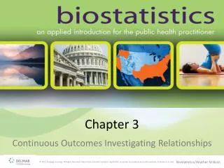
Continuous Outcomes Making Comparisons. Chapter 2. Outline. Describing: Numerical summaries Graphical summaries One-Sample comparisons: Historical controls Paired differences Two-Sample comparisons: Equal variances Unequal variances Multiple-Sample comparisons: ANOVA

E N D
Continuous Outcomes Making Comparisons Chapter 2
Outline • Describing: Numerical summaries Graphical summaries • One-Sample comparisons: Historical controls Paired differences • Two-Sample comparisons: Equal variances Unequal variances • Multiple-Sample comparisons: ANOVA Multiple comparisons
Continuous Outcomes • No gaps: All values are possible. Level of detail is limited only by measurement tool. • Examples: Blood pressure Weight Hemoglobin Concentrations Gene expression levels
Learning Objectives • How do I describe continuous data? • How do I make comparisons? • How do I make comparisons when the distribution is not symmetric? • How do I plan for a study when the outcome is continuous and I need to make a comparison?
Public Health Application The US EPA estimates that 76 – 85 million pounds of atrazine (6-chloro-N2-ethyl-N4-isopropyl-1,3,4-triazine-2,4-diamine), a triazine herbicide, is produced annually with approximately 76.5 million pounds applied within the United States. Atrazine’smain use is to control broadleaf and grassy weeds with the most common sites of application being corn, sugarcane, and sorghum. Once introduced into the environment, atrazine is not easily broken down and has been shown to persist for long periods. This persistence provides ample opportunity for water system contamination (Agency for Toxic Substances and Disease Registry 2003). Current research shows that atrazine exposure may pose a significant threat to human health with drinking water providing the most widespread route of water.
Data Description • Longitudinal study conducted to investigate the effects of drinking water exposed to herbicides and maternal health outcomes: 979 pregnant women with data at week 9: • 270 drank only tap water during pregnancy • 315 drank only bottle/filtered water during pregnancy • 394 drank a combination of tap and bottle/filtered water Demographic variables collected at week 9 Hemoglobin measured throughout pregnancy
Research Question Does exposure to herbicides in drinking water impact changes in hemoglobin?
Describing the Data • Numerical summaries: Common measures of center and spread • Graphical summaries: Histograms Box-and-whisker plots Mean plots (with error bars)
Most Important Step in Data Analysis • Describe the data: Before making conclusions or inferences, an investigator needs to fully understand what the data looks like. • Numerical and graphical summaries cannot be skipped! Need this information to choose the most appropriate statistical method Need this information for valid statistical inferences
Numerical Summaries • Continuous variables are described by reporting summaries for the center and the spread. • Center: Mean Median • Spread: Variance or standard deviation Range or interquartile range (IQR)
Summary of the Center • Mean: Most often reported Sum of observations divided by the number of subjects May not be robust to extreme observations • Median: Often reported when the outcome is not normally distributed Observations are sorted, represents the middle observation More robust to extreme observations
Summary of the Spread • Variance/ standard deviation: Reported with the mean Summarizes how much deviation there is from the mean Standard deviation is the square root of the variance • Range/interquartile range: Reported with the median Range: Difference between the largest and the smallest observations Interquartile range: Range of middle 50% of observations
Summary of the Center: Mean • The mean is the sum of all the values divided by the total number of subjects. • The mean of the population is a parameter. • The mean of the sample is a statistic.
Summary of the Center: Median Sort all the observations from smallest to largest; the median is the value in the middle. The median represents the 50th percentile of the data since 50% of the observations are smaller and 50% of the observations are larger. The median of the population is a parameter. The median of the sample is a statistic.
Summary of the Spread: Variance Deviations from the mean • The variance is the average squared deviation from the mean. The variance of the population is a parameter. The variance of the sample is a statistic.
Summary of the Spread: Standard Deviation • Standard deviation is the square root of the variance. Square root of the variance units are the same as the mean of standard deviation is often reported. The standard deviation of the population is a parameter. The standard deviation of the sample is a statistic.
Which Distribution has the Larger Variance (or Standard Deviation)?
Summary of the Spread: Range • The range is the difference between the largest and smallest values. Although the range is an actual number, it is often reported as an interval (minimum, maximum). The range of the population is a parameter. The range of the sample is a statistic.
Summary of the Spread: Quartiles • First quartile: Median of the first half of the sorted observations (sorted smallest to largest) Represents the 25th percentile • Third quartile: Median of the last half of the sorted observations (sorted smallest to largest) Represents the 75th percentile • The difference between the first and third quartiles is the IQR.
Summary of Spread: IQR • The IQR is the difference between the 25th percentile and the 75th percentile values. Although the IQR is an actual number, it is often reported as an interval (first quartile, third quartile). The IQR of the population is a parameter. The IQR of the sample is a statistic. • IQR provides a range for the middle of the data. 50% of the observations fall within the IQR.
Summary of the Spread: Five-Number Summary Minimum: Smallest value First quartile: 25th percentile value Median: Middle or 50th percentile value Third quartile: 75th percentile value Maximum: Largest value
Which is Better?Range vs IQR • Unlike the variance and the standard deviation, the range and the IQR give different information. If the goal is to understand the spread of all observations, the range is better. The range can appear larger if there are extreme observations that do not “fit” with the rest. The IQR provides the range of observations for the middle.
Histograms • Provide a picture of the shape of the distribution: Peaks Symmetry Spread Center Extreme values
Box-and-Whisker Plots Graphical representation of the five-number summary Useful only if there are groups to compare
Mean Plots (Error Bars) • Mean plots are the bar graphs where the height of the bar represents the size of the mean. • Error bars are often included: Standard deviation error bars for understanding the spread in the sample Standard error error bars for making inferences
Summary Histograms are helpful for describing the shape of a distribution. Box-and-whisker plots can be used for comparing the distribution between groups. Means plots provide a graphical comparison of means. Numerical and graphical summaries are essential for describing continuous variables.
Description of the Sample • A sample of pregnant women exposed to herbicides in drinking water: 270 women drank only tap water during pregnancy • Tend to be young (average age 25 years, SD = 1.9) • Report a median household income of $33K with a range of $8.7K • Have a low educational attainment (only 45% have a high school degree)
Why a One-Sample Study? • Obtaining an additional group or sample for comparisons may not be practical. Comparisons involve historical control(s). • The change/difference is of interest. Variability between subjects is too large to make meaningful comparisons. Paired differences.
Historical Controls • Want to compare what you found in the sample with something: Do your results differ from what has been previously published/reported? • Historical controls: Control data are not collected concurrently within the same study. • Different time period • A different region • Different population • Different kind of exposure • Seems economical—why not use historical controls all the time?
Paired Differences • Subjects in the sample serve as their own control: Having an independent control group does not provide a good comparison. More variability is expected between subjects. Subjects are too different to make useful comparisons. • Examples
One-Sample StudyHemoglobin Change • Historical control: Do pregnant women exposed to herbicides have the same mean hemoglobin change as women exposed to mercury ? Mean hemoglobin change in pregnant women exposed to mercury has been reported as 2.0 g/dL. • Paired difference: Do pregnant women exposed to herbicides have a mean change in hemoglobin? Mean change different from 0 g/dL would suggest a change.
Inferences for the One-Sample Study • Hypothesis tests Assume the null parameter is the true parameter • Historical control study: Null parameter = Historical value • Paired difference study: Null parameter = 0 Decide whether the data support this assumption • Confidence intervals Estimate the true parameter using interval Can use the interval estimate to determine if assumptions about the parameter are reasonable
Inferences for the One-Sample StudyHistorical Controls Research hypothesis: The true mean () hemoglobin change for pregnant women exposed to herbicides is not 2.0 g/dL. Null hypothesis: The true mean () hemoglobin change for pregnant women exposed to herbicides is 2.0 g/dL.
Inferences for the One-Sample StudyPaired Differences Research hypothesis: The true mean () hemoglobin change for pregnant women exposed to herbicides is not 0 g/dL. Null hypothesis: The true mean () hemoglobin change for pregnant women exposed to herbicides is 0 g/dL.
One-Sample StudyHemoglobin Change • The outcome is hemoglobin change; so, the two types of one-sample studies seem similar. True Outcome is change; so, the only difference is the null parameter (2 g/dL or 0 g/dL). If the outcome is not a change, the tests are still similar, but historical control does not require a paired difference.
Planning • Estimation: Width of the interval Amount of variability • Comparison of means: Power Significance level Effect size
Nonparametric Tests • The hypothesis tests and confidence intervals assumed that the outcome was normally distributed. What if this is not reasonable? What if the mean is not a good summary of the center? • Nonparametric tests allow for comparisons without assuming the outcome is normally distributed.
Signed Rank Test Research hypothesis: The hemoglobin values for week 9 and week 36 have different distributions. Null hypothesis: The hemoglobin values for week 9 and week 36 have the same distribution. Essentially, a one-sample hypothesis test about the median instead of the mean.