Download
1 / 57
570 likes | 729 Vues
Standard genetic simplex models in the classical twin design with phenotype to E transmission Conor Dolan & Janneke de Kort Biological Psychology, VU. Two general approaches to longitudinal modeling Markov models: (Vector) autoregressive models for continuous data

E N D
Standard genetic simplex models in the classical twin design with phenotype to E transmission Conor Dolan & Janneke de Kort Biological Psychology, VU
Two general approaches to longitudinal modeling Markov models: (Vector) autoregressive models for continuous data (Hidden) Markov transition models discrete data (Mixtures thereof) Growth curve models (Brad Verhulst, Lindon Eaves): Focus on linear and non-linear growth curves Typically multilevel or random effects model (Mixtures thereof) Which to use? Use the model that fit the theory / data / hypotheses
First order autoregression model. A (quasi) simplex model (var(e)>0). zx zx zx b2,1 b3,2 b4,3 x1 x2 x3 x4 1 1 1 1 y1 y2 y3 y4 1 1 1 1 e2 e3 e1 e4 b03 b02 b01 b04 1
First order autoregression model. A quasi simplex model (var(e)>0). zx zx zx b2,1 b3,2 b4,3 x1 x2 x3 x4 1 1 1 1 y1 y2 y3 y4 1 1 1 1 e2 e3 e1 e4 yti = b0t + xti + eti x1i = x1i= zx1i xti = bt-1,t xt-1i + zxti var(y1) = var(x1) + var(e1) var(xt) = bt-1,t2var(xt) + var(zxt) cov(xt,xt-1) = bt-1,tvar(xt)
First order autoregression model. A quasi simplex model (var(e)>0). zx zx zx b2,1 b3,2 b4,3 x1 x2 x3 x4 1 1 1 1 y1 y2 y3 y4 1 1 1 1 e2 e3 e1 e4 Identification issue: var(e1) and var(et) are not identified. Solution set to zero, or equate var(e1) = var(e2) , var(e3) = var(e4)
var(y1) = var(x1) + var(e1) var(xt) = bt-1,t2var(xt) + var(zxt) cov(xt,xt-1) = bt-1,tvar(xt) Standardized stats I: Reliability at each t, rel(t) : rel(x1) = var(x1) / {var(x1) + var(e1)} Interpretation: % of variance in y at t due to latent x at t
var(y1) = var(x1) + var(e1) var(xt) = bt-1,t2var(xt) + var(zxt) cov(xt,xt-1) = bt-1,tvar(xt) Standardized stats II: Stability at each t,t-1, stab(t,t-1): bt-1,t2var(xt) / {bt-1,t2var(xt) + var(zxt)} Interpretation: % of the variance in x at t explained by regression on x at t-1 (latent level!)
var(y1) = var(x1) + var(e1) var(xt) = bt-1,t2var(xt) + var(zxt) cov(xt,xt-1) = bt-1,tvar(xt) Standardized stats III: Correlation t,t-1, cor(t,t-1): bt-1,t2var(xt) / {sd(yt-1) * sd(yt)} sd(yt) = sqrt(var(xt) + var(et)) var(xt) = bt-1,t2var(xt) + var(zxt) Interpretation: strength of linear relationship
.288 .288 .288 zx zx zx .8 .8 .8 .8 x1 x2 x3 x4 1 1 1 1 y1 y2 y3 y4 1 1 1 1 .2 .2 .2 .2 e2 e3 e1 e4 1.0000 0.6400 1.000 0.51200.6401.000 0.40960.5120.640 1.0000
Special case: factor model var(zxt) (t=2,3,4) = 0 b2,1 b3,2 b4,3 x1 x2 x3 x4 1 1 1 1 y1 y2 y3 y4 1 1 1 1 e2 e3 e1 e4 x1 b2,1 b3,2b4,3 1 b2,1 y1 y2 y3 y4 b2,1b3,2 1 1 1 1 e2 e3 e1 e4
1.0000 0.6400 1.000 0.51200.640 1.000 0.40960.5120.640 1.0000 var(zxt) (t=2,3,4) = 0 1.000 0.758 1.000 0.705 0.668 1.000 0.640 0.607 0.564 1.000
Multivariate decomposition of phenotypic covariance matrix: Sph = SA + SC + SE Sph1 Sph12 Sph2 = SA + SC + SE rSA+ SC + SESA + SC + SE
Sph = SA+ SC + SE Estimate SA using a Cholesky-decomp SA = DADAt DA = d110 0 0 d21 d22 0 0 d31 d32 d33 0 d41 d42 d43 d44
Sph = SA+ SC + SE Model SA a simplex model SA = (I-B)A YA (I-B)At + QA
SA = (I-BA) YA (I-BA)t + QA BA = 0 0 0 0 bA21 0 0 0 0 bA32 0 0 0 0 bA43 0
SA = (I-BA) YA (I-BA)t + QA YA = var(A1) 0 0 0 0 var(zA2) 0 0 0 0 var(zA3) 0 0 0 0 var(zA4)
SA = (I-BA) YA (I-BA)t + QA QA = var(a1) 0 0 0 0 var(a2) 0 0 0 0 var(a3) 0 0 0 0 var(a4)
zA2 zA3 zA4 bA3,2 bA4,3 bA2,1 A1 A2 A3 A4 1 1 1 1 A1 A2 A3 A4 1 1 1 1 a2 a3 a1 a4 The genetic simplex (note my scaling)
zA zA zA A11 A12 A13 A14 1 y11 y12 y13 y14 zE zE zE 1 E11 E12 E13 E14 1 zC zC zC C1 C2 C3 C4 1 E21 E22 E23 E24 1 zE zE zE y21 y22 y23 y24 1 A21 A22 A23 A24 zA zA zA
zA A12 a2 c2 y12 zE e2 E12 Occasion specific effects zC C2 a2 E22 zE c2 y22 e2 A22 zA
Question: h2, c2, and e2 at each time point? var(yt) = {var(At) + var(at)} + {var(Ct) + var(ct)}+ {var(Et) + var(et)} h2= {var(At) + var(at)} / var(yt) c2= {var(Ct) + var(ct)} / var(yt) e2= {var(Et) + var(et)} / var(yt) zA A12 a2 c2 y12 zE e2 E12 zC C2
Question: contributions to stability t-1 to t bAt-1,t2var(At) / {bAt-1,t2var(At) + var(zAt)+var(at)} bCt-1,t2var(Ct) / {bCt-1,t2var(Ct) + var(zCt)+var(ct} bEt-1,t2var(Et) / {bEt-1,t2var(Et) + var(zEt)+var(et)} zA zA A13 A14 y13 y14 zE zE E13 E14 zC zC C3 C4
Question: contributions to stability t-1 to t {bAt-1,t2var(At)+bCt-1,t2var(Ct)+bEt-1,t2var(Et)} [{bAt-1,t2var(At) + var(zAt)+var(at)} + {bCt-1,t2var(Ct) + var(zCt)+var(ct} +{bEt-1,t2var(Et) + var(zEt)+var(et)}] Decompose the phenotypic covariance into A,C,E components
Birley et al. Behav Genet 2005 (alternative: growth curve modeling)
Nivard et al, 2014 Anx/dep stability due to A and E from 3y to 63 years
zA zA zA A11 A12 A13 A14 1 y11 y12 y13 y14 zE zE zE 1 E11 E12 E13 E14 1 zC zC zC C1 C2 C3 C4 1 E21 E22 E23 E24 1 zE zE zE y21 y22 y23 y24 1 A21 A22 A23 A24 zA zA zA Phenotype-to-phenotype transmission (Eaves etal. 1986)
zA zA zA A11 A12 A13 A14 1 y11 y12 y13 y14 zE zE zE 1 E11 E12 E13 E14 1 zC zC zC C1 C2 C3 C4 1 E21 E22 E23 E24 1 zE zE zE y21 y22 y23 y24 1 A21 A22 A23 A24 zA zA zA Sibling “interaction” mutual direct phenotypic influence (Eaves, 1976; Carey, 1986)
a a a A A A A y y y y e e e E E E E c c c C C C C E E E E e e e y y y y A A A A a a a Niching picking (Eaves et al., 1977)
a a a A A A A a1 a2 a3 y y y y e e e E E E E b2 b3 b1 c c c C C C C E E E E b1 b2 b3 e e e a1 a2 a3 y y y y A A A A a a a Niching picking (Eaves et al., 1977)
“Niche-picking” During development children seek out and create and are furnished surrounding (E) that fit their phenotype. A smart child growing up will pick the niche that fits her/her phenotypic intelligence. A anxious child growing up may pick out the niche that least aggrevates his / her phenotypic anxiety. Phenotype of twin 1 at time t -> environment of twin 1 at time t+1 (parameters at)
Mutual influences During development children’s behavior may contribute to the environment of their siblings. A smart child growing up will pick the niche that fits her/her phenotypic intelligence and in so doing may influence (contriibute to) the environment of his or her sibling. A behavior of an anxious child may be a source of stress for his or her siblings. Phenotype of twin 1 at time t -> environment of twin 2 at time t+1(parameters bt)
ACE simplex T=4 Identification in ACE simplex with no additional constraints. Except: Occasion specific residual variance decomposition: Var[y(t)|A(t), E(t), C(t)] = var[e(t)] Var[e(t)] = var[a(t)]+var[e(t)], t=1,…,4
Identification #1 T=4 phtiE(t+1)j (i=j) phtiE(t+1)j(i≠j) a1, a2, a3b1, b2, b3 (not ID) a1, a2=a3b1, b2=b3 ak=b0a+(k-1)*b1a bk=b0b+(k-1)*b1b (k=1,2,3) but a1=a2,a3b1= b2,b3 (not ID) Presence of C not relevant to this results Good…..?
a a a A A A A a1 a2 a3 y y y y e e e E E E E b2 b3 b1 c c c C C C C E E E E b1 b2 b3 e e e a1 a2 a3 y y y y A A A A a a a
N required given plausible values ACEa1, a2=a3 & b1, b2=b3 akbk ~N (power=.80) .10 .10 11700 .10 .15 4700 .15 .10 12100 .15 .15 4800 Hypothesis: a1=a2=a3=0 & b1= b2=b3 =0 (4df) Good....?
zA zA zA A11 A12 A13 A14 1 y*11 y*12 y*13 y*14 a1 a3 a2 E zE zE 1 b1 b2 b3 E11 E12 E13 E14 1 zC zC zC Not Good! C1 C2 C3 C4 1 E21 E22 E23 E24 b1 1 b2 b3 zE zE zE a3 a1 a2 y*21 y*22 y*23 y*24 1 A21 A22 A23 A24 zA zA zA
zA zA zA A11 A12 A13 A14 1 y*11 y*12 y*13 y*14 a2 a3 a1 zE zE zE 1 b1 b2 b3 E11 E12 E13 E14 E21 E22 E23 E24 b3 b2 b1 1 zE zE zE a1 a2 a3 y*21 y*22 y*23 y*24 1 A21 A22 A23 A24 zA zA zA
N required given plausible values AEa1, a2=a3 & b1, b2=b3 akbk~N (power=.80) .10 .10 620 .10 .15 260 .15 .10 580 .15 .15 240 Good...? Hypothesis: a1=a2=a3=0 & b1= b2=b3 =0 (4df)
True AE+ak& bk (Nmz=Ndz=1000) akbkACE simplex df=61 .10 .10 5.44 .10 .15 11.22 .15 .10 5.62 .10 .15 11.54 Good...? (approximate model equivalence)
zA zA zA A11 A12 A13 A14 1 y*11 y*12 y*13 y*14 a2 a3 a1 zE zE zE 1 b1 b2 b3 E11 E12 E13 E14 E21 E22 E23 E24 b3 b2 b1 1 zE zE zE a1 a2 a3 y*21 y*22 y*23 y*24 1 A21 A22 A23 A24 zA zA zA
Full scale IQ. 261 MZ and 301 DZ twin pairs. mean (std) ages 5.5y (.30), 6.8y (.19), 9.7y (.43), and 12.2y (.24). The proportions of observed FSIQ data 0.812, 0.295, 0.490, 0.828 (MZ twin 1) 0.812, 0.295, 0.490, 0.828 (MZ twin 2) 0.774, 0.379, 0.598, 0.797 (DZ twin1) 0.774, 0.379, 0.598, 0.797 (DZ twin 2)
5.5y6.8y9.7y12.2y 0.7700.6740.8400.802 MZ FSIQ correlation 0.6410.4820.4810.500 DZ FSIQ correlation Red: MZ stdevs Green: DZ stdevs
Fitted standard simplex Var(at) = zero time specific A zero Var(zA3) = var(zA4) = 0 A inno at t=3,4 zero Chi2(63) = 76.8, p= 0.11
OPEN ACCESS • Dolan, C.V, Janneke M. de Kort, Kees-Jan Kan, C. E. M. van Beijsterveldt, Meike Bartels and Dorret I. Boomsma (2014). Can GE-covariance originating in phenotype to environment transmission account for the Flynn effect? Journal ofIntelligence. Submitted. Dolan, C.V., Johanna M. de Kort, Toos C.E.M. van Beijsterveldt, Meike Bartels, & Dorret I. Boomsma (2014). GE Covariance through phenotype to environment transmission: an assessment in longitudinal twin data and application to childhood anxiety. Beh. Gen. In Press.
A A A A A A A 1 y y y y a2 a3 a1 E E E 1 b1 b2 b3 E E E E E E E E b2 b3 b1 1 E E E a1 a2 a3 y y y y 1 A A A A A A A