Download
1 / 60
740 likes | 1.19k Vues
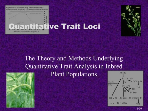
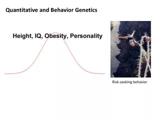
Quantitative genetics: traits controlled my many loci. Key questions: what controls the rate of adaptation? Example: will organisms adapt to increasing temperatures or longer droughts fast enough to avoid extinction? What is the genetic basis of complex traits with continuous variation?.

E N D
Quantitative genetics: traits controlled my many loci Key questions: what controls the rate of adaptation? Example: will organisms adapt to increasing temperatures or longer droughts fast enough to avoid extinction? What is the genetic basis of complex traits with continuous variation?
Breeder’s equation Breeder’s equation: R = h2S
LOCUS TRAIT A Z1 B # of individuals C D Z E F Polygenic Inheritance Leads to a Quantitative Trait
Problems in predicting the evolution of quantitative traits • Dominance • Epistasis • Environmental effects
Environment alters gene expression - epigenetics yellow: no difference; red or green = difference age 3 age 50
Major questions in quantitative genetics • How much phenotypic variation is due to genes, and how much to the environment? • How much of the genetic variation is due to genes of large effect, and how much to genes of small effect?
Measuring heritability Variance: _ Vp= Σi (Xi – X)2 --------------- (N – 1)
Variance components VP = total phenotypic variance VP = VA + VD + VE + VGXE VA = Additive genetic variance VD = Dominance genetic variance (non- additive – can include epistasis) VE = Variance among individuals experiencing different environments VGXE = Variance due to environmental variation that influences gene expression (not covered in text)
Heritability = h2 = VA / VPThe proportion of phenotypic variance due to additive genetic variance among individuals h2 = VA / (VA + VD + VE + VGXE) Heritability can be low due to:
Additive vs. dominance variance Additive: heterozygote is intermediate Dominance: heterozygote is closer to one homozygote (Difference from line is due to dominance)
Dominance Genotype Toe len (cm) AA 0.5 AA’ 1.0 A’A’ 1.0 f(A) = p = 0.5 f(A’) = q = 0.5 Start in HWE f(AA) = 0.25 f(AA’) = 0.50 f(A’A’) = 0.25 Codominant (additive) Genotype Toe len (cm) AA 0.5 AA’ 0.75 A’A’ 1.0 f(A) = p = 0.5 f(A’) = q = 0.5 Start in HWE f(AA) = 0.25 f(AA’) = 0.50 f(A’A’) = 0.25 Dominance and heritability
Codominant (additive) Dominance Dominance and heritability II Starting Genotype frequencies Genotype Genotype Mean = 0.75 cm Mean = 0.875 cm Starting Phenotype frequencies Phenotype (toe len – cm) Phenotype (toe len – cm)
Additive Dominance Select toe length = 1 cm Starting Genotype frequencies Genotype Genotype Mean = 1.0 cm Mean = 1.0 cm Starting Phenotype frequencies S = Phenotype (toe len – cm) Phenotype (toe len – cm) S =
Codominant (additive) Dominance Effects of dominance: genotypes after random mating Genotype freq after selection, before mating Genotype Genotype Genotype freq after mating Genotype Genotype
Codominant (additive) Dominance Effects of dominance: phenotypes after random mating Phenotype freq after selection, before mating Genotype mean = 0.954 mean = 1.0 Phenotype freq after mating R=1 - .75 = 0.25 R = 954 - .875 = 0.079 Phenotype Phenotype
Dominant S = R = R = h2S h2 = R / S = Codominant (additive) S = R = R = h2S h2 = Effect of dominance on heritability
Agouti is antagonist for MC1R. If agouti binds, no dark pigment produced agouti MC1 MC1-receptor Second problem predicting outcome of selection: epistasis Example: hair color in mammals
MC1-receptor Normal receptor Mutant: never dark pigment (yellow labs) Mutant: always dark pigment Second problem predicting outcome of selection: epistasis Epistasis agouti MC1
Epistasis example Genotype Phenotype EE / AA dark tips, light band ee / -- blond / gold / red Ed- / -- all dark EE / Ad- blond / gold / red Want dark fur: population ee / AA Ee / AdA Ee / AA
Epistasis example ii Cross: Ee / AdA x Ee / AdA genotype phenotype freq EE / AdAd 1/16 EE / AdA 1/8 EE / AA 1/16 Ee / AdAd 1/8 Ee / AdA 1/4 Ee / AA 1/8 ee / AdAd 1/16 ee / AdA 1/8 ee / AA 1/16
Estimating h2 Analysis of related individuals Measuring the response of a population, in the next generation, to selection
Heritability is estimated as the slope of the least-squares regression line
h2 example: Darwin’s finches mean before selection: 9.4 mean after selection: 10.1 S = 10.1 - 9.4 = 0.7
h2 example: Darwin’s finches II mean before selection: 9.4 mean of offspring after selection: 9.7 Response to selection: 9.7 – 9.4 = 0.3 R = h2S; 0.3 = h2 * 0.7 h2 = R/S = 0.3 / 0.7 = 0.43
Controlling for environmental effects on beak size • song sparrows: cross fostering Offspring vs. biological parent (h2); vs. foster parent (VE) Smith and Dhondt (1980)
Testing for environmental effects How can we determine the effect of the environment on the phenotype?
Two genotypes in two environments: possible effects on phenotype
Environmental effects: carpenter ant castes major worker minor worker queen male
Effect of GxE: predicting outcome of selection 7 yarrow (Achillea millefolium) genotypes 2 gardens Clausen, Keck, and Heisey (1948)
Gen. 2 Gen. 1 Gen. 0 freq. trait, z Modes of selection
freq. freq. trait, z trait, z Mode of selection: directional
freq. freq. trait, z trait, z Mode of selection: stabilizing
freq. freq. trait, z trait, z Mode of selection: disruptive
Disruptive selection Distribution of mandible widths in juveniles that died (shaded) and survived (black)
Beak width Beak depth Fitness Beak depth Fitness Beak width Complications: correlations • Darwin’s finches: beak width is correlated with beak depth
QTLs and genes of major effects How important are genes of major effect in adaptation?
QTL analysis: Quantitative Trait Loci – where are the genes contributing to quantitative traits? • Approach • two lineages consistently differing for trait of interest (preferably inbred for homozygosity) • Identify genetic markers specific to each lineage (eg microsatellite markers) • make crosses to form F1 • generate F2s and measure trait of interest • test for association between markers and trait • Estimate the effect on the phenotype of each marker
Example: Mimulus cardinalis and Mimulus lewisii Mimulus cardinalis Mimulus lewisii