Sequencing and Sequence Alignment

1. Sequencing and Sequence Alignment CIS 667 Bioinformatics Spring 2004

2. Protein Sequencing • Before DNA sequencing, protein sequencing was common • Sanger won a Nobel prize for determining amino acid sequence of insulin • Protein sequences much shorter than today’s DNA fragments • One amino acid at a time can be removed from the protein • The aa can then be determined

3. Protein Sequencing • Unfortunately, this works only for a few aa’s from the end • So insulin broken up into fragments Gly Ile Val Glu Ile Val Glu Gln Gln Cys Cys Ala

4. Protein Sequencing • Then the fragments are sequenced • After they are assembled by finding the overlapping regions Gly Ile Val Glu Ile Val Glu Gln Gln Cys Cys Ala Gly Ile Val Glu Gln Cys Cys Ala

5. Protein Sequencing • By the late 1960s protein sequencing machines on market • RNA sequencing following the same basic methodology by 1965

6. DNA Sequencing • DNA was first sequenced by transcribing DNA to RNA • Slow - years to sequence tens of base pairs • By mid 70s Maxam and Gilbert learned how to cleave DNA selectively at A, C, G, or T • This led to the development of Maxam-Gilbert sequencing method

7. Maxam-Gilbert Sequencing • Single-stranded DNA labeled with radioactive tag at 5’ end • Sample quartered and digested in four base-specific reactions • Reaction concentrations are such that each strand of DNA in each sample cut once at random location • Use gel electrophoresis to find lengths of tagged fragments

9. Sanger Sequencing • Today, an alternative method called Sanger sequencing is generally used • A primer bonds to a single-stranded DNA near the 3’ end of the target to be sequenced • DNA polymerase extends the primer along the target DNA • For each of the 4 bases this extension is done

10. Sanger Sequencing • A small amount of extension ending nucleotides are introduced • This causes the extension to end randomly at a specific base • Now use gel electrophoresis and read the sequence as the complement of the bases

11. Sanger Sequencing

12. Sequence Alignment • Given two string, find the optimal alignment of the strings • Strings may be of different lengths, optimal alignment may include gaps • An alignment score is produced Example: SHALL WEAR ALL WE SHALL WEAR --ALL WE--

13. Sequence Alignment • Alignment score produced by looking at each column in alignment • Match gives column a +1 score • Mismatch: -1 • Space: -2 HELLO THERE JELLO TEAR- Score: 7*(+1)+3*(-1)+1*(-2)=2

14. Sequence Alignment • In biology, the sequences to be aligned consist of nucleotides or amino acids • Sufficiently similar sequences can allow us to infer homology • Common evolutionary history • We can also infer the function of a protein or gene given similarity to one with known functionality

15. Sequence Alignment • Since homologous sequences share a common evolutionary history the alignment score should reflect evolutionary processes • DNA changes over time due to mutations • Most mutations are harmful • May be due to environmental factors, e.g. radiation

16. Mutation • May also be due to problems in the transcription process • One nucleotide may be substituted for another • Deletion of a nucleotide • Duplication • Insertions • Inversions

17. Mutation

18. Mutation • Deletions have different effects depending on the number of nucleotides deleted • Deletions of 3 in an ORF result in the deletion of a codon, so an amino acid is not produced • Usually damaging, sometimes lethal • Deletion of 1 causes a frame shift - changes all downstream amino acids • Almost always lethal

19. START IPTYGI STOP START IPTYI STOP Codon Deletion ATGATACCGACGTACGGCATTTAA ATGATACCGACGTACGGCATTTAA

20. START IPT STOP START IPTYGI STOP Frame Shift ATGATACCGACGTACGGCATTTAA

21. Mutations • Some notes… • A single base substitution may even produce the same amino acid (especially if it is the last in a codon) • May also produce a similar amino acid • It is impossible to tell whether the gap in an alignment results from insertion in one sequence or deletion from another • After mutation, an organism may be more or less likely to survive natural selection

22. Alignment Scores • Based on what we have said about mutations - how should we modify the alignment scores? • Note that a single long gap is more likely than several shorter ones… • Therefore it should have a smaller penalty • Say… • Match: +1 • Mismatch: 0 • Gap origination: -2 • Gap extension: -1

23. Alignment • We can have sequences with different sizes • An alignment is defined to be the insertion of spaces in arbitrary locations along the sequences so that they end up being the same size • No space in the sequence can be aligned with a space in the other GA-CGGATTAG GATCGGAATAG

24. Alignment • Let’s use the following scores for similarity - match: +1; mismatch: -1; space: -2 • Let sim(s, t) denote the similarity score for two sequences s and t • We want to develop an algorithm to compute the maximum sim(s, t) given s and t

25. Dynamic Programming • We will use a technique known as dynamic programming • Solve an instance of a problem by using an already solved smaller instance of the same problem • In our case, we build up the solution by determining the similarities between arbitrary prefixes of the two sequences • Start with shorter prefixes, work towards longer ones

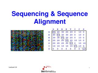
26. Dynamic Programming • Let m be the size of s and n the size of t • Then there are m + 1 prefixes of s and n + 1 prefixes of t, including the empty string • We store the similarities of the prefixes in an (m + 1)  (n + 1) array • Entry (I, j) contains the similarity between s[1..I] and t[1..j]

27. Dynamic Programming • Let s = AAAC and t = AGC • We need to initialize part of the array to get started • If one of the sequences is empty, we just add as many spaces as characters in the other sequence • Correspondingly, we fill in the first row and column with multiples of the space penalty (-2)

28. Dynamic Programming • We can compute the value of entry (i, j) by looking at just three previous entries: (i - 1, j), (i - 1, j - 1), (i, j - 1) • Corresponds to these choices • Align s[1..i] with t[1..j - 1] and match a space with t[j] • Align s[1..i - 1] with t[1..j - 1] and match s[i] with t[j] • Align s[1..i - 1] with t[1..j] and match s[i] with a space

29. Dynamic Programming • If we compute entries in an smart way, scores for best alignments between smaller prefixes have already been stored in the array, so sim(s[1..i], t[1..j] = max {sim (s[1..i], t[1..j - 1]) - 2, sim (s[1..i - 1], t[1..j - 1]) + p(i, j), sim (s[1..i - 1], t[1..j]) - 2} Where p(i, j) = + 1 if s[i] = t[j], -1 otherwise

30. Dynamic Programming • We should fill in the array row by row, left to right • If we denote the array by a then we have a[i, j] = max {a[i, j - 1] - 2, a[i - 1, j - 1] + p(i, j), a[i - 1, j] - 2} Where p(i, j) = + 1 if s[i] = t[j], -1 otherwise

31. Dynamic Programming Algorithm Similarity input:sequences s and t output: similarity of s and t m  |s| n  |t| for i  0 to m do a[i, 0]  i  g for j  0 to n do a[0, j]  j  g for i  1 to m do for j  1 to n do a[i, j]  max(a[i - 1, j] + g, a[i - 1, j - 1] + p(i, j), a[i, j - 1] + g) return a[m, n]

32. Optimal Alignments • So now we know the maximum similarity, but we still need to compute the optimal alignment • We will use the array a of similarities previously computed • To be continued …