Download
1 / 48
500 likes | 778 Vues
Frequency Analysis. Fourier analysis deals with the representation of signals by sinewave components. The simplest type of Fourier analysis is that of the Fourier series where a periodic signal x(t) is represented as a sum of sinewaves.

E N D
Fourier analysis deals with the representation of signals by sinewave components. The simplest type of Fourier analysis is that of the Fourier series where a periodic signal x(t)is represented as a sumof sinewaves.
The sinewaves could be sin (), cos () or a combination thereof: The sinewave components in the summation will be a complex sinewave at various frequencies:
The complex sinewave frequencies are integral multiples of Where T is the period of the signal to be represented.
The resultant summation is a weighted sum of the complex sinewaves ejw0t: The weights or coefficients Xn are found from
The weights Xn correspond to the magnitudes of the frequency components of the spectrum of x(t). X(f) X0 X-1 X1 X-2 X2 X-3 X3 . . . . . . f -3w0 -2w0 -w0 w0 2w0 3w0
Example: Find the Fourier series for the following function: x(t) . . . . . . t T
Solution: this function is clearly periodic. We calculate the coefficients as follows:
X(f) . . . . . . f f0
Example: Find the Fourier series for the following function: T 1 -1 Solution: The coefficients are calculated in much the same way as before.
The spectrum of the squarewave is shown below |X(f)| 1 1 . . . . . . f -5f0 -3f0 -f0 f0 3f0 5f0
Fourier Transforms Fourier transforms allow the frequency analysis of non-periodic as well as periodic functions. The Fourier transformation is derived from Fourier series. To derive the Fourier transform, let us take the Fourier series, and take the limit as T As T, we also have w00 (since w0=2p/T).
This last expression is a Riemann sum which is a definite integral: where f = nDf. Using this last piece of notation in X(nDf), we have
This last expression is the definition of the Fourier transform of x(t):
In the process of deriving and expression for the Fourier transform, we have also derived an expression for the inverse Fourier transformation:
Example: find the Fourier transform of a delta function, x(t)=d(t). d(t) t Solution: using the definition of the Fourier transform, we have
As corollary of this last problem, we have the following: the inverse Fourier transformation of one is a delta function: This will be a very useful fact in other Fourier transform derivations.
F F {d(t)} d(t) 1 F -1 f t We know that the Fourier transform of a delta function is one. What is the Fourier transform of one? The answer may be obtained by noticing the similarities between the forward transformation and the reverse transformation.
Let us do a few manipulations on the inverse Fourier transformation:
Thus we have the Fourier transform of a Fourier transform: If we know the forward Fourier transform, we can find the reverse Fourier transform. This property is called duality.
Applying this result to the Fourier transform of d(t), we have A physical interpretation can be given to the Fourier transforms of d(t) and 1. The function 1 is a D.C. signal whose sole frequency component is 0 Hz. This component is represented by a spike at 0 rad/sec in the frequency domain. The function d(t) is like a lighting bolt whose spectrum covers the entire frequency band (from f = 0 to ).
Suppose we had a function x(t) whose Fourier transform we know, X(f). We then wished to know the Fourier transform of a shifted version of x(t), x(t-a):
Applying this principle to F {d(t)}, we have Using duality, we also have
The previous two results could also have been had by direct application of the Fourier transform:
As a corollary of the previous Fourier transformations, we also have A summary of the Fourier transforms derived so far are shown in the table on the following slide.
The plots of these Fourier transforms are shown below. d(f+f0) d(f-f0) F {cos 2pf0t} f jd(f+f0) F {sin 2pf0t} jd(f-f0) f
The physical interpretation of these transforms should be clear: the spectrum of a sinewave consists of spikes at the frequency of the sinewave along with a spike at the corresponding negative frequency. The (generally complex) coefficients of the spikes depend upon the phaseof the sinewave.
Now, let’s find the Fourier transform of a pulse: x(t) t -½ ½ This function is sometimes referred to as P(t) . Applying the definition of the Fourier transform, we have
Exercise: find the Fourier transform of the following pulsed sinewave: