Download

1 / 44
480 likes | 687 Vues
Natural Neighbor Based Grid DEM Construction Using a GPU. Thomas Mølhave Duke University. Joint work with Pankaj K. Agarwal and Alex Beutel. Flood mapping – Mandø , Denmark. 90 meter grid resolution. 2 meter grid resolution. LIDAR – Light Detection and Ranging.

E N D
Natural Neighbor Based Grid DEM Construction Using a GPU Thomas Mølhave Duke University Joint work with Pankaj K. Agarwal and Alex Beutel
Flood mapping – Mandø, Denmark 90 meter grid resolution 2 meter grid resolution
LIDAR – Light Detection and Ranging Source: http://minnesota.publicradio.org/display/web/2008/07/09/digitalmap/
Digital Elevation Model (DEM) • Geographic Information Systems need models • Enables many applications • Hydrology, contouring, noise computations, line- of sight, city planning
Digital Elevation Models • Triangular Irregular Network (TIN) 4
GRID Terrain Models • Interpolation • Linear interpolation based on Delaunay triangulation [Agarwal et al. ‘05] • Simple but not smooth • Relatively fast • Regularized spline with tension (RST) [Mitasovaet al. 93] • Uses high-order polynomials • Better with sparse data • Slow
Natural Neighbor Interpolation (NNI) • Based on Voronoi Diagram • Has been used • Slow implementations NNI Linear Interpolation
Voronoi Diagram A Voronoi cell Vor(pi) is the region in space for which pi is the closest point (the nearest neighbor) from the set of input points S
Natural Neighbor Interpolation • Vor(q) takes area from neighboring cells (natural neighbors) • Interpolate h(q) based on weighted average of heights of natural neighbors h(pi) • Weights are based on:
Our Contributions • Build high-quality, large-scale grid DEMs with a natural neighbor based interpolation scheme using the GPU • Handle gaps in data by introducing the idea of region of influence • Tuned for interpolating on uniform grid. Handle 106 NNI queries in one “pass”. Previous maximum of ~32 [Fan etal. ‘05] • Use CUDA to improve performance
Outline • GPU background • Voronoi diagrams • NNI in one point • Batched NNI • NNI for grids • More Parallelism • Evaluation
Graphics Processing Unit (GPU) • Specialized hardware for parallel processing • Render 3D objects on 2D plane of pixels from a viewpoint o • Not just for graphics: • Robot collision detection, database systems, fluid dynamics
GPU Buffers Color Buffer • Buffers are 2D array of pixels. • Color Buffer • Stores information about color as seen from viewpoint • Can blend objects • bitwise-OR • Depth buffer • Stores distance to closest object from viewpoint • Can be set to read-only
GPU Model of Computation FAST CPU Main Memory SLOW FAST GPU Graphics Card Memory
Computing the Voronoi Diagram [Hoff, et al. 1999]
Voronoi Diagram and Lower Envelopes • For each point pi define function • Lower envelope of {f1,f2…fn} is • Lower envelope is distance from x to its nearest neighbor
Rendering the Voronoi Diagram Render on GPU with looking at cones from below (viewpoint at -∞)
PixelizedVoronoi Diagram • Drawing on GPU discretizes Voronoi diagram. Call this PVorS(p). • Render cone for each input point • Depth buffer stores distance from the pixel to the closest input point (structure of the Voronoidiagrmam) • Color buffer can store any information specific to the closest input point Depth Buffer Color buffer
Generating PixelizedVoronoi Diagrams Render using truncated polyhedralcones
Truncated PixelizedVoronoi DiagramTPVor(S) • Radius of cone r defines region of influence • If two points are >2r apart their cones can not overlap and they can not effect each other.
Natural Neighbor Interpolation [Fan, et al. ’05]
Natural Neighbor Interpolation • Vor(q) takes area from neighboring cells (natural neighbors) • Interpolate h(q) based on weighted average of heights of natural neighbors h(pi) • Weights are based on:
Natural Neighbor Interpolation Discrete version: Area of new Voronoi Cell: Interpolated value: |TPVor(q1)| = 73 h(q1)=(33/73)h(p1)+(12/73)h(p2)+(28/73)h(p3) Call this process BufferAnalysis
NNI Query Processing Main Memory GPU Memory
Batching NNI Queries [Fan, et al. ’05]
Batching NNI Queries • For a given pixel, only need to know if Voronoi cell for q covers it (Y/N) • Only use one bit in color buffer for each query • Color buffer performs bitwise-OR
NNI for Grid DEM Construction Grid of queries, MxMgrid
Batched NNI on Grids • w is number of bits in color buffer (and number of queries we can handle by previous algorithm) • Break grid into query blocks of size B x B • Could handle each in one pass with previous algorithm
Batched NNI on Grids • Assumptions: • Queries in same position in different query blocks are independent • Execute previous algorithm on each query block simultaneously
Larger Grids • Grids restricted by size of memory on GPU • Use I/O-efficient partitioning • recursion depth
Implementation • Ran on • Intel Core2 Duo CPU running Ubuntu 10.4 • NVIDIA GeForce GTX 470 with CUDA 3.0 • OpenGL • TemplatedPortable I/O Environment (TPIE) for interacting with disk efficiently
NNI Batch Query Processing • Optimize GPU to CPU communication • Transferring color buffers between GPU and CPU memory is slow • For each query we have a multiple pixels • Transferring extra data • Perform BufferAnalysis with CUDA directly on GPU • Only transfer one value for each query point SLOW SLOW
Tests • Afghanistan: • 3.5 gigabytes • 186 million data points • 4 km2region • Fort Leonard Wood (Missouri) • 57 GB • 2.2 billion data points • 600 km2region Source: NASA Data from the Army Research Office
Performance - Efficiency Times in seconds
Performance - Efficiency Times in seconds
Performance - Efficiency Times in seconds
Performance - Quality Afghanistan all ground points Afghanistan sparse ground points NNI Linear Interpolation
Future Work • Make region of influence more flexible • Extend algorithm to 3D • Spatial-temporal data
Thank you Thanks to the Army Research Office for access to data