Download
1 / 12
120 likes | 326 Vues
Gaussian PDF Cloud Parameterization. Peter Caldwell, Steve Klein, Sungsu Park + you. Outline: The PDF Macrophysics Microphysics Future work (radiation, ice, variance, convection). PDF: Formulation. Using a bivariate Gaussian in T l and q w =q t - q l

E N D
Gaussian PDF Cloud Parameterization Peter Caldwell, Steve Klein, Sungsu Park + you Outline: • The PDF • Macrophysics • Microphysics • Future work (radiation, ice, variance, convection)
PDF: Formulation • Using a bivariate Gaussian in Tl and qw=qt-ql • follows Sommeria+Deardorff (1977), Mellor (1977) • qwPDF for liquid only. Ice follows default CAM5. • imperfect: ice inconsistency persists, qw not conserved. • Can be rewritten as univariate Gaussian in S=qw’ – BlTl’ where Bl=δqs/δT|Tl • univariatealways used for calculation • bivariateness only meaningful if σTl and σqw have real meaning • note if ql>0, ql=S+Q where Q=qw-qs(Tl,p)
PDF: Variance • CAM5 cloud frac uses triangular PDF in qt with half-width δ ∝ Rhcrit • Currently spoof CAM5 by using triangle’s variance. • Tldependence requires an approximation. • Future work=diagnostic, process-based variance. 0.8 Rhcrit Profile δ 400mb { 700mb qt qs { CAM5 Our scheme 0.79 0.89 land ocn
Macrophysics: Formulation • Computing liquid cloud fraction Al and cell-aveql from the S PDF is straightforward: • CAM5 uses triangular distn for Al and implicit, conserved Zhang et al (2003) for ql (+checks). Fig: Example PDF from ASTEX (dots) with Gaussian fit (line) and cldfrac(shaded).
Macrophysics: Results • cldfrac changes explained by param rather than feedbacks. • generally small changes.
Macrophysics: Understanding CldFrac PDF Run PDF ‘parasite’ off CAM5 run CAM5 Run Fig: 850 mbliquid cloud fraction (LCLOUD) from 1 mo CAM simulations. • PDF-forced and PDF-parasite runs similardifferences from cldfracparam • Cloud fraction differences due (partly?) to making width ∝ qw rather than qs. Fig: Cloud fraction vs qt/qs(T,p) for Gaussian, CAM5 (triangular), and Gaussian using CAM5 qs approach at p=500 mb, T=240 K.
Microphysics: Subgrid ql For microphysical process w/ local rate R=xqly: autoconversion, accretion, immersion freezing, contact freezing, sedimentation • CAM5: • assumes SGS ql variability follows Γdistn • for given ql, drop diameter D follows a Γdistn with params chosen to keep drop conc constant • Gaussian PDF: • local ql=S+Q ql follows truncated Gaussian distn. 1d table lookup
Microphysics: Substepping • Most of CAM5 microphysics is substepped, requiring PDF updates. • Updated PDF is Gaussian with unchanged Al and ql matching that prognosed by the model. • this approach makes qlpdf inconsistent with S PDF. • conceptually, this means that condensation/evaporation only occurs during macrophysics… which is logical. • Updating can be done by simply calingμ and σ by α=ql,new/ql,old! • If ql,old=0, Al and ql PDF equations can back out params. • Updated rates could be calculated as old rate times αy
Microphysics: Results Accretion: Autoconversion: note scale change! Immersion Freezing: (Contact freezing always 0) • Using old/new agreement to test for bugs • At first glance, scheme looks reasonable!
Microphysics: Results • Rates often agree, but many cases where parasite >driver exist. Fig: Autoconversion rates (color) as a function of ql and Nd. The RHS panel shows % difference between Gauss and Gamma rates (with denom chosen as min{driver,parasite} to emphasize errors). The RHS panel uses 2 runs (Gauss-driven and Gamma-driven) to increase the number of data points.
Microphysics: Results Discrepancies aren’t correlated with height or whether all water was used up in the timestep. Fig: Gauss – Gamma % difference (prev slide RHS) broken into cases where microphysics depletes all ql (so limiting is needed) or not. Symbol size ∝ pressure level.
Microphysics: Results Is difference explained by PDF shapes? Fig: Gauss – Gamma % difference (prev slide RHS) broken into cases where microphysics depletes all ql (so limiting is needed) or not. Symbol size ∝ pressure level.