Download
1 / 22
250 likes | 515 Vues
Visual ModelQ Training. Building a PI controller. This unit discusses Installation of Visual ModelQ The Visual ModelQ default model Placing and configuring blocks Wiring a model Compiling and running a model. Install Visual ModelQ. To run Visual ModelQ the first time:.

E N D
Visual ModelQ Training Building a PI controller • This unit discusses • Installation of Visual ModelQ • The Visual ModelQ default model • Placing and configuring blocks • Wiring a model • Compiling and running a model
Install Visual ModelQ To run Visual ModelQ the first time: • Click here to visit www.QxDesign.com • Download Visual ModelQ** • Run Visual ModelQ installation • Launch Visual ModelQ using the Windows start button or clicking on the icon • The “default model” should appear **This unit can be completed with a free (unregistered) copy of Visual ModelQ
The default model • The default model has two required elements, a Solver and a Scope. It also includes a square-wave generator wired to a 1-Channel Live Scope. Click Run to compile and run this model. Square-wave generator Run button Wire connecting generator output to scope input Live Scope displays on model canvas
Modify the default model • Stop the model using the stop button or the escape key. • Select (click on) and delete the 1-Channel Live Scope.
Move Wave Gen • Move the waveform generator to the left to make room. We’ll use this block to generate the command.
Add 2-Channel Live Scope • Add a 2-Channel Live Scope. We’ll use this to compare the command and feedback signals. Click on the icon in the circle; place as indicated by the arrow.
Add a subtraction block • Place a subtraction block on the model canvas. We’ll use this block to form the error, the difference between the command and the feedback signals.
Add PI Control Law • Add a PI (Proportional-Integral) Control Law from the “Analog” tab. The PI controller is popular in industry because it’s simple and it provides good performance in most systems.
Add Power Converter Model • Add a 2-pole low-pass filter from the “Analog” tab to simulate the effect of power conversion. All control systems have power converters and a low-pass filter is often a good model.
Configure the Power Converter • Set the frequency of the low-pass filter to 800 Hz to simulate an 800 Hz bandwidth converter. Double-click on the Frequency node of the filter (in red circle) to view adjustment window.
Add Plant Scaling • Add a “Scale-by” block from the “Math” tab to simulate the gain of the “plant.” All plants have gain. Examples of plant gain are inertia of a motor and inductance of a coil.
Add Integral • Add an integral from the “Analog” tab to simulate an integrator in the plant. The integrating plant is the most common plant in industrial control systems. ` The plant model is a combination of a gain block and an integral.
Add Live Constants • Add 3 Live Constants from the “Constants” tab; these gains will be easy to change while the model runs. Change the names to KP, KI, and System Gain (double-click in strings under blocks). Double-click in this area to change name.
Flip Live Constants • Flip the constants KI and System Gain; this will make wiring more convenient. Right click inside each block and select “Flip Horizontal” from the pop-up menu.
Initialize Live Constants • Set initial gains as KP = 2, KI = 100, and System Gain = 500. Set these gains by double-clicking on the diamond in the upper left corner (shown by red circles) to get initialization window.
Wire the Model • Select the wiring icon. • Connect 11 wires as below. Move mouse over a node and click to start a wire; move to second node and click again to finish. Example: move mouse to one end and click to start a wire; move to the other end and click again.
Save the Model • Click “File, Save…” or use the file save icon. • Save as “Building a PI Controller”
Compile the Model • Click the compile button. When the model compiles, the button changes from red to green and a grid is drawn in the Live Scope.
Set the Scope Scaling • Double-click on Live Scope for control panel. Set Channel 1 scaling to 0.5; repeat for Channel 2. Set Time to 0.01.
Set the Scope Trigger • Select Trigger Tab of Live Scope control panel. Select Normal trigger.
Run the Model • Click the run button. The Live Scope compares command (blue) to feedback (red). The values of KP(2) and KI (100) provide good performance; settling time is ~15 mSec with little overshoot.
Visit www.QxDesign.com for information about software and practical books on controls. Click here for information on Visual ModelQ Click here for information on Observers in Control Systems, published by Academic Press in 2002 Click here for information on Control System Design Guide (2nd Ed.), published by Academic Press in 2000