Download
1 / 22
220 likes | 304 Vues
Learn the basics of binomial distribution using a scenario with Graphics Calculators. Understand the formula, parameters, and various probability scenarios. Explore examples to grasp concepts clearly and enhance your understanding of probability distributions.

E N D
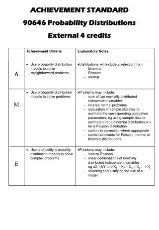
ACHIEVEMENT STANDARD 90646 Probability Distributions External 4 credits
Intro to Binomial Distribution The probability that a Graphics Calculator is faulty is 0.01 We have 5 GC left to sell at school. • What is the probability that NO GC are faulty? • What is the probability that 1 GC is faulty? • What is the Probability that 2 GC are faulty? • What is the probability that 3 GC are faulty? • What is the probability that 4 GC are faulty? • What is the probability that 5 GC are faulty? The probability of “x” faulty =
Binomial Distribution • A random variable X has a BINOMIAL DISTRIBUTION if: • F: There are a fixed number of trials (n) • 2: There are only 2 outcomes – success and failure • I: Each trial is independent • C: The probability of success, p, of each trial is constant. • e.g. the number of sixes scored when you throw a dice 10 times has a binomial distribution because: • There are a fixed number of trials (10) • There are only 2 outcomes – either you get a 6 or you don’t. • Each trial is independent – whatever you get on one throw does not affect the outcome on the next throw • The probability of getting a six (1/6) does not change during the 10 throws. The binomial probability formula is: P(X = x) = nCx px(1-p)n-x The two parameters are n (no of trials) and p (prob of success) On GC: Stat/Dist/Binm. Bpd means: Binomial P(x = a) Bcd means: Binomial P(x ≤ a) (cumulative from x = 0 up to and including x = a, i.e. x = 0, 1, 2, 3… a) Terms: No more than 7 = 0,1,2,3,…7 = P(X ≤ 7) Less than 7 = 0,1,2,…6 = P(X ≤ 6) At least 7 = 7,8,9,… = P(X ≥ 7) = 1 – P(X ≤ 6) More than 7 = 8,9,10… = P(X ≥ 8) = 1 – P(X ≤ 7) FOR ANY QUESTION THAT asks for the prob that X “is more than b” or “at least b” turn the qn into 1 – P(X ≤ c) where the c is the biggest number NOT INCLUDED
Some Binomial examples: • E.g. 1 A dice is thrown 10 times and the number of sixes scored is recorded. • Find the probability that 4 of the 10 throws landed on a six • Find the probability that none of the throws landed on a six • Find the probability that at least one throw landed on a six • E.g. 2 a) A survey shows that 25% of households use Colgate toothpaste. In a sample of 10 households, what is the probability of finding exactly 2 households that use Colgate toothpaste? • Find the probability that more than 4 of the 10 households use Colgate toothpaste. Extra notes space if needed:
Binomial Distribution – combined events Recall: if two events are independent then: P(A and B) = P(A) x P(B) One of the conditions of the Binomial distribution is that the events are independent. So if we are working out the probability of two or more events occurring we just multiply their probabilities. • e.g. The probability that Kobe makes a free throw shot is 0.83. Assume that each attempt at a free throw is independent of another. • Kobe takes 10 free throws in a game • Calculate the probability that he makes at least 6 out of the 10 free throws. • Kobe takes 10 free throws in the next game also. • b) Calculate the probability that he makes at least 6 out of 10 free throws in both games • c) Calculate the probability that he makes half his free throws in one game and all his free throws in the other game
Binomial Distribution Harder questions This is not required for level 3 – but scholarship students should know how to do this. Recall the formula is P(X = x) = nCx px(1-p)n-x Or you can use the tables on the formula sheet E.g. The probability that a torpedo from a submarine hits its target is 45%. The target must be hit at least 3 times to be destroyed. How many torpedoes should be fired to give the submarine a 90% chance of sinking the target. We are trying to find n with p = 0.45 and P(x ≥ 3) = 0.9. Therefore P(X ≤ 2) = 0.1. E.g.2 Faxes that are sent to a travel shop are either local or overseas. If the probability that out of 10 faxes, none are from overseas is 0.01, find the probability that a fax coming in is from overseas.
Poisson Distribution Named after mathematician Simeon-Denis Poisson 1781-1840 • The Poisson Distribution measures how many times a discrete event happens over a continuous time interval. • Compare with Binomial which looks at how many successes over a fixed number of trials(so in Binomial there is a limit to what the value of X can be… in the Poisson there isn’t). • Examples of Poisson Distributions: • The number of cars passing through an intersection per hour • How many patients a doctor sees per hour • How many misprintsper page in a newspaper Conditions that need to be met for Poisson Distribution: C R I S P R events must occur at Random I events must be Independent of each other S events cannot occur Simultaneously P probability of an event occurring is Proportional to the size of the time interval GC: stat/dist/Poisn Ppd = Poisson with P(X=x) Pcd = Poisson with P(X ≤ a). Note: You will need to convert questions that have P(X≥ a)or P (X > a) into 1 – P(x ≤ b) as with the Binomial.
Poisson Distribution The distribution is given as: P(X = x) = e-λλx x! Parameter: λ = the mean number of occurrences per time period Or use Graphics Calc using X and λ (λ = rate or average) E.g. The number of babies born at Christchurch Women’s Hospital is estimated to be 6 per day. Assume that the Poisson distribution can be used to model this distribution a) Find the probability that on a randomly selected day there are no births at Christchurch Women’s Hospital. b) Find the probability there are no more than 3 babies born on a given day c) Find the probability that there are at least 5 babies born on a randomly chosen day. If the question refers to a different time period (e.g babies born per hour) then you need to adjust the rate so it matches the question (ie daily rate ÷ 24). This is based on the assumption of the Poisson distribution that the prob of an event occuring is proportional to the size of the interval d) Find the probability that no babies are born in one particular hour? e) Find the probability that in two one-hour periods 1 baby is born in each
Poisson Distribution – working backwards Sometimes you need to use the formula: P(X = x) = e-λλx x! Or the tables from the formula sheet to answer questions Note: If they ask to find the “mean” or “average” this is the same as the rate… i.e λ Usually you need to find a value for the p(x=0) and substitute these (x = 0, and p) into the formula, then use GC Solver to find λ E.g.1 In samples of material taken form a textile factory, 40% had at least one fault. Estimate the mean number of faults per sample. E.g. 2 Assume that samples are independent. Calculate the probability that two randomly chosen samples both have no faults.
Normal Distribution The Normal Distribution is a continuous distribution (unlike Binomial and Poisson). We relate the probability to an interval rather than a specific value. To find P(x1<X<x2) we find the area under the curve from x1 to x2 The normal distribution formula is (you don’t need to know this!): F(x) = 1 e-(x-μ)2/2σ2 √2πσ2 The two parameters are the mean μ and std dev σ. Standardised Normal Distribution Since every different context will have different values of μ and σ we use a “standardised normal distribution” (Z) which converts a number from it’s original value (X) into a Z-value which measures the number of std dev this x value is away from the mean: Z = X – μ σ This standardised distn has μ = 0, σ = 1 In context μ - σ μ μ + σ Std normal 1 0 1
Normal Distribution cont • Some basics you need to know about the normal dist: • It is symmetrical about the y axis • The area under the curve is equal to one • The curve approaches the x axis asymptotically – it extends to infinity in both directions ALWAYS draw a diagram to represent the problem • To solve normal distribution problems you need to know: • The mean μ • The standard deviation σ. • To find the required probability you can either use: • Graphics Calc: STAT DIST NORM Ncd • Normal Distribution Tables (formula sheet): these require you to convert to Z values (std normal) using Z = (X – μ) / σ first.
Solving Problems using Normal Dist • Always draw diagram to represent problem. • Label the mean and std dev on diagram • Shade the area you are interested in. e.g. weights of Y13 students are normally distributed with a mean of 65kg and a standard deviation of 12kg. Find the probability that a Y13 student chosen at random weighs more than 60kg. Draw diagram: Using GC • Go to STAT DIST NORM then Ncd • Lower = Upper = σ = μ = • Calc • P(X > 60) =
More Solving simple problems using Normal Dist • e.g. weights of Y13 students are normally distributed with a mean of 65kg and a standard deviation of 12kg. • Find the probability that a student chosen at random weighs between 60kg and 75kg • Find the probability that a student chosen at random weighs less than 55kg a) Draw diagram to show P(60 < x < 75) b) Draw diagram to show P( x < 55) Using GC: Upper limit = Lower limit = Mean = Std dev = P(60 < x < 75) = Using GC:
Inverse Normal Problems - Merit Sometime we are given problems where we know the probability and need to find the random variable (x), the mean μ or the std dev σ. In this case use the CG InvN The InvN button calculates the X value if you already have the mean (μ) and theprobability (area) of getting a value LESS THAN X (as shown in the diagram below): E.g. A battery manufacturer has found that their AA batteries have a mean lifetime of 5 hours and a std dev of 0.4 hours. The manufacturer wants to guarantee that they will last for X hours and wants the claim to be correct for 95% of the batteries produced. What number of hours should he claim? 1. DRAW DIAGRAM! GC: InvN Area = σ = μ = X = Claim:
Inverse Normal Problems cont - Merit • If the problem requires you to find the mean μ: • you will need to first find a z-value (the number of std devs away from the mean). To do this use InvN with the required area, mean = 0 and std dev = 1. This gives you the z-value (as opposed to an X-value). • then use the formula z = (X- μ)/ σ and Solver to find the mean μ • e.g.The expected life of a small turtle has a std dev of 2 years. The probability that a randomly chosen turtle’s life exceeds 28 years is 0.03. Assume their lifetimes are normally distributed. • Find the mean life time. • Find the expected values between which 90% of all turtles can be expected to live DIAGRAM • Use InvN with area = ____, μ = ____, σ = ____ • gives z = _______. • Use formula z = (x- μ)/ σ and solver to find μ: • Find P(x1<X<x2) = 0.90 Diagram: • For x1 use InvN with area = _____, μ = ____, σ = ____ • X1 = • For x2 use InvN with area = _____, μ = ____, σ = ____ • X2 =
Continuity Correction • We use the continuity correction if: • The data is discrete (e.g test scores) • The data is being measured to the nearest unit (eg to the nearest kg) • Using the normal to approximate the Poisson or Binomial which are discrete. • To use the cont. corr. focus on the end points and change them so that the continuous interval includes the original discrete end points. e.g. Sacks of potatoes are filled by a machine. The weight of potatoes in each sack (to the nearest kg) is normally distributed with a mean of 60kg and std dev of 4kg. a) Find the probability that a randomly selected sack weighs more than 65kg. b) Find the probability that a sack weighs between 57kg and 62kg. a) Draw diagram b) Draw diagram b) P( < X < ) a) Need P(x > )
Combined Events for Poisson, Normal or Binomial (merit / excel) If events are independent (which is the assumption for all of these distributions) then the probability of one event and then another (same or different) event occurring in a row is: P(first event) x P(second event) since P(A∩B) = P(A) x P(B) E.g.1 A long-life bulb has a life which is normally distributed withy mean of 2400 hours and std dev of 150 hours. 2 randomly selected bulbs are chosen. Calculate the probability that both will last longer than 2500 hours. P(X > 2500) using GC (normal dist, Ncd) = So prob that both = E.g. 2. In a factory producing t-shirts, the chance of a t-shirt having a fault is 5%. If two samples of 10 shirts are taken what is the probability that there are no faults in one sample and at least one fault in the other sample? Binomial distribution with n = , p = P(X = 0) = so therefore P(X > 0) = So P(no faults first sample, at least one in second sample) = And P(at least one fault first sample, no faults in second sample)= Therefore P(no faults in one sample and at least one fault in the other sample)
Calculating the parameters from raw data (M/E) Sometimes we could be given the raw data and need to calculate the parameters before we can answer the question. Parameters are the statistics needed to describe the distribution. The parameters for each distribution are listed below: Binomial: No of trials, Prob of success (n and p). To find p from raw data calculate: Poisson: The rate or average per period (λ) Normal: Mean and std dev (μ and σ) To find the rate λ(for the Poisson), or the mean and std dev for Normal enter the data into a list in the GC.. See below: The table shows the number of birds nests per hectare • To find the average number of birds nests per hectare: • In GC/Stat enter the data into list 1 and list 2 respectively • Choose CALC, SET and check XList says List 1 and Freq says List2. • Choose 1var • The average is the mean x • If you need the std dev choose xσn
Sum of two Independent Normal Distributions (Merit) Say we have two normal distributions X1 and X2. X1 has mean μ1 and std dev σ1 and X2 and mean μ2 and std dev σ2 Then for the sum of the two normal distributions (X1 + X2) mean of (X1 + X2)=μ1 + μ2 variance of (X1 + X2) = Var(X1) + Var(X2) = (σ1)2 + (σ2)2 std dev of (X1 + X2) = √ (σ1)2 + (σ2)2 ALSO for thedifferenceof the two distributions(X1 - X2) mean of (X1 - X2)=μ1 - μ2 variance of (X1 - X2) = Var(X1) + Var(X2) = (σ1)2 + (σ2)2 std dev of (X1 + X2) = √ (σ1)2 + (σ2)2 So to calc std dev – find variances first, add them and take square root Note that we subtract the means but add vars Be careful not to confuse these two situations: T = 3X and T = x1 + x2 + x3 The first one is a constant (3) multiplied by one variable The second one is three variables added together Var(3X) = 32Var(X) so SD(3X) = 3SD(X) Var(x1 + x2 + x3) = Var(X1) + Var(X2) + Var(X3) so SD = √3var(X) = √3 SD(X) (assuming each variable has the same VAR and are independent)
Sum of two Independent Normal Distributions (Merit) continued • E.g. In a manufacturing plant tins of spaghetti are produced. The weight of the cans are normally distributed with a mean of 75g and a std dev of 8g. The spaghetti that goes inside the cans is also normally distributed with a mean of 380g and a std dev of 35g. • The quality control officer inspects the total weight of the product once the can is filled with spaghetti. • Calculate the mean and std dev of the total weight of the can and spaghetti together. • b) The manufacturer aims to have most filled cans weighing over 375g. Calculate the proportion of filled cans that do not meet this aim. ASSUMPTION: The two distributions are INDEPENDENT
Linear Combinations of Normal Distributions (Excellence) As before, say we have two normal distributions X1 and X2. X1 has mean μ1 and std dev σ1 and X2 and mean μ2 and std dev σ2 If T = aX1 + bX2 Then Mean (T) = a μ1 + b μ2 Variance (T) = a2Var(X1) + b2Var(X2) = a2 σ12 + b2 σ22 Std dev (T) = √ a2 σ12 + b2 σ22 Also for a combination of more than two independent normally distributed random variables: Let Y = x1 + x2 + x3 + … Xn Then mean (Y) = μ1 + μ2 + μ3 + … + μn std dev (Y) = √(σ12+ σ22 + σ32 +… + σn2 ) ASSUMPTION: Events must be independent
Linear Combinations of Normal Distributions (Excellence) cont E.g. A lift has a maximum load of 1050kg. The weight of an adult man is normally distributed with a mean of 77kg and a std dev of 9kg. If 13 adult men get on the lift, find the probability that the lift is overloaded.