Download
1 / 14
140 likes | 279 Vues
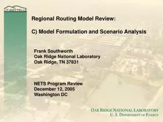
Regional Routing Model Review: C) Model Formulation and Scenario Analysis. Frank Southworth Oak Ridge National Laboratory Oak Ridge, TN 37831 NETS Program Review December 12, 2005 Washington DC. Calibration. Changes in Demands. Network Changes. Transit times, distances.

E N D
Regional Routing Model Review: C) Model Formulation and Scenario Analysis Frank Southworth Oak Ridge National Laboratory Oak Ridge, TN 37831 NETS Program Review December 12, 2005 Washington DC
Calibration Changes in Demands Network Changes Transit times, distances County/Port Based Commodity Production /Consumption Forecasts County/Port Based Mode/Route/Market Choice Model(s)* Changes to Network Conditions (Capacities) and Mode/Route Costs Forecasting, Scenario Analysis dollar/ton shipment rates NETS Tier 1 Regional Economic Activity Forecasts/ Scenarios Mode Specific Rate Estimation Models Forecast / Scenario Based Commodity Flows, Costs and Benefits Fuel, labor, I&M costs by vehicle /vessel types (C,M,V) (Data) Changes in Supply Calibration, Forecasting & Scenario Analysis Base Case Computed Flows, Costs (and Benefits) * = Simultaneous or nested mode and destination choice linked to capacity constrained route assignment
Estimate Commodity Production (O) & Consumption (D) by Region Estimate O-to-D Costs per Ton Connect Os and Ds to Estimate O-to-D Commodity Flows Assign O-to-D Flows to Modes & Routes Iterate to Convergence Re-Estimate O-to-D Costs per Ton Re-Estimate O-to-D Flows The Basic Flow and Cost Estimation Process
Prototype Regional Routing Model Formulation: + m 1/ βm ( Xi jm ln Xi jm) + m 1/ λm ( Xi jkm ln Xi jkm) subject to: Vak = ∑i ∑j ∑r δ i,j akr X i j kr for all links, a, and modes k, in the network ∑rX i j rk = X i j k for i=1,2,...I, and j=1,2,...J ∑kX i j k = X i j for i=1,2,...I, and j=1,2,...J Vak ≥ 0 X i j kr ≥ 0 V = a link volume X = an O-D flow volume S = link transportation time or generalized cost
i j m ] Aim Bjm Xi jm = Oi m Dj m F[ βm, * m i j ( Xi jm di j m } / i,j Xi jm = Freight Destination Choice (Flows Modeling): where i j m ]} for all i Aim = 1/{j Bjm Djm F [ βm, Bj m = 1/{i Aim Oim F [ βm, i j m ]} for all j and
c ijm = -(1/ λm ) ln {k exp (-λm c i j km )} Freight Mode Choice: Xijkm = Xijm *[exp(-θm ckm)/ ∑kεK(m) exp(-θm ckm)] where (for example): cijkm = α0 + α1 rijkm + α2 Sijkm + α3 vijkm and, (links mode and destination choice)
Components of Freight Costs that Need Modeling: Number of different “legs” to a journey Shipper/receiver perceived costs per leg: freight rate transit time service reliability Congestion effects i.e. congestion transit time and reliability direct plus indirect (i.e. rate) effects on costs
Lock Congestion Function 19 2000 2000 18.5 1800 1800 18 1600 1600 17.5 S = S0 * (1+ 0.15 (V/C)**4) 1400 1400 S = k /((C/x) – – 1) 17 1200 1200 S=Travel Time (Minutes) 16.5 S= Minutes of Delay/Tow 1000 1000 16 800 800 15.5 600 600 15 400 400 14.5 200 200 k k 14 0 0 5 5 10 10 15 15 20 20 25 25 30 30 35 35 40 40 45 45 50 50 0 500 1000 1500 2000 C/2 C/2 C C Traffic Volume (Vehicles/hour) x =Kilotons/Year (in thousands) Network Link Transit Time (Congestion) Functions Highway Congestion Function “Generic” link congestion function for use in Toy Model: Sa = Sao * [ 1 + θ1* Va + θ2 *( Va / Capa)γ ]
Generalized Transportation Costs (Shipper Perspective) Level 1: (Statistical) Freight Rates In-Transit Times Service Quality (Reliability) Level 2: (Engineering) Variable Operating Costs (Annualized) Capital Operating Costs Line-haul costs Loading/unloading costs Equipment utilization costs Commodity carrying costs Administrative costs Shipment distance Cargo type (commodity, weight, volume) Labor rate Fuel price Carrier/operator type Equipment type Company type (private/for-hire; size) Contract type (duration) Facility type, Location, Operating licenses, fees and taxes Components of Freight Movement Costs
35 41 Port C 36 38 37 10 33 8 2 39 7 32 42 44 11 27 29 16 25 Port B 12 Lock c Lock b 1 14 43 28 23 26 9 15 24 13 40 3 Port A 6 17 Lock a 31 34 18 30 19 Key: 20 Network Nodes (44) 40 5 Traffic Centroids (10 in all) 4 21 Links (110 in all): 22 Truck Rail Inland Water Deep Water
7 8 2 9 1 3 6 4 5
Model Run # 1 Origin Mode Split = 36.7% water 63.3 % rail
Model Run # 2 Origin Mode Split = 74.9% water 25.1% rail