Download
1 / 39
450 likes | 515 Vues
The Course of Synoptic Meteorology. MUSTANSIRIYAH UNIVERSITY COLLEGE OF SCIENCES ATMOSPHERIC SCIENCES DEPARTMENT 2018-2019 Dr. Sama Khalid Mohammed SECOND STAGE. Welcome Students In The New Course and In The First Lecture . What are covered in this course?. Introduction

E N D
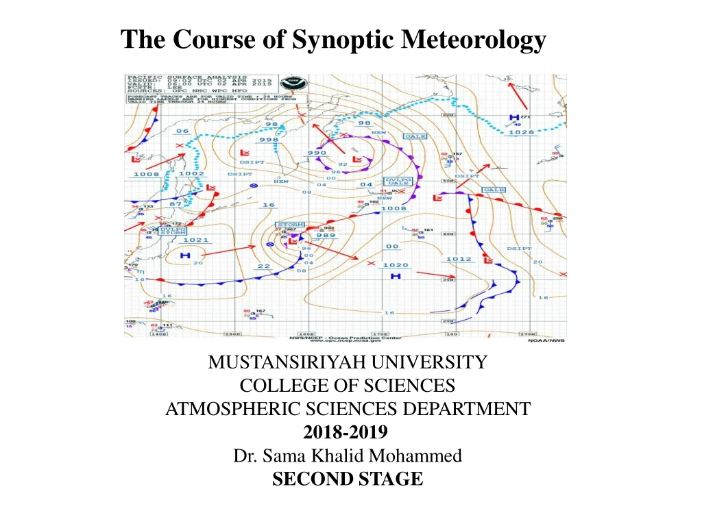
The Course of Synoptic Meteorology MUSTANSIRIYAH UNIVERSITY COLLEGE OF SCIENCES ATMOSPHERIC SCIENCES DEPARTMENT 2018-2019 Dr. Sama Khalid Mohammed SECOND STAGE
Welcome Students In The New Course and In The First Lecture
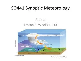
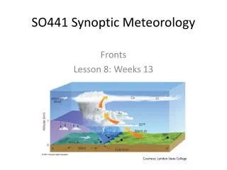
What are covered in this course? Introduction Scales of Atmospheric Motion, Synoptic Meteorology, Analysis and interpretation. Weather Maps Surface maps and upper air maps in addition to Upper air code . Contouring Weather Maps Contour lines and types, pressure analysis, Low and high pressure systems and their extensions, discontinuity, waves. Air Masses Types of air masses, formation methods of air masses, prevailing air masses, thermal inversions. Fronts Introduction, warm front, warm front circulation, cold front, cold front circulation, horizontal and vertical structure of cold front, frontal theory, rule of locating fronts on weather maps. Life Time of Frontal Low Classical model, Structure of open wave, subtropical and polar jet streams. Jet Stream Definition, its types (subtropical and polar jet streams).
References G., Lackmann,2011:MidlatitudeSynopticMeteorologyDynamics, Analysis & Forecasting, American Meteorological Society, 345 p. C.D.,Ahrens, 2008:Essentials of Meteorology. Thomson Brooks/Cole, 504 p. A., Lehkonen, 2013: Synoptic Meteorology, Eumetrain, 190 p. https://www.meted.ucar.edu/index.php منعم الجبوري وسناء عبدالجبار، 2010 :تجارب عملیة في الرصد والتحلیل والتنبؤ. مؤسسة مصر – مرتضى، بغداد. 284 ص.
Introduction • Synoptic: from “Synoptikos”, a Greek word, means “presenting a summary of the principal parts or a general view of the whole” or “view together”. • in Synoptic, all information concerning the state of the troposphere is taken into account: observations and the parameters produced by numerical models. • For us, Synopticmeans that you take everything you learned from physical meteorology, dynamic meteorology, remote sensing, and put them together. • Synoptic will help a meteorologist to understand the state of the troposphere; what is happening and why, and what might be taking place in the near future. • Synoptic meteorology traditionally involves the study of weather systems, such as high and low pressure systems, jet streams and associated waves, and fronts.
Scales of Atmospheric Motion The Atmosphere is the mass of air surrounding the earth and bound to it more or less permanently by the earth's gravitational attraction, and is the most unstable part of the climate system, and its processes contribute to the variability of the climate system on a wide range of spatial and temporal scales. Meteorologists arrange circulations according to their size, start from tiny gusts to giant storms which is called the scales of motion. • Consider smoke rising into the clean air from a chimney in the industrial section of a large city. Within the smoke, small chaotic motion (tiny eddies) cause it to tumble and turn. These eddies constitute the smallest scale of motion ”The Microscale”, in which eddies have diameters of a few meters or less and they form by convection or by the wind blowing past obstructions and are usually short-lived, lasting only a few minutes at best.
As the smoke rises, it drifts toward the centerof town. Here the smoke rises even higher and is carried back toward the industrial section. This circulation of city air constitutes the next larger scale “The mesoscale” (meaning middle scale). Typical mesoscale winds range from a few kilometers to about a hundred kilometers in diameter. Generally, they last longer than microscale motions, often many minutes, hours, or in some cases as long as a day. Mesoscalecirculations include local winds (which form along shorelines and mountains), as well as thunderstorms, tornadoes, and small tropical storms.
When we look for the chimney on a surface weather map, neither the chimney nor the circulation of city air shows up. All that we see are the circulations around high and low pressure areas. We are now looking at the synoptic scale, or weather map scale or cyclonic scale(a scale at which atmospheric phenomena at horizontal dimensions that are much larger than their vertical dimensions. It is the typical weather map scale that shows features such as high- and low pressure areas and fronts over a distance spanning a continent). Circulations of this magnitude dominate regions of hundreds to even thousands of square kilometres and, although the life spans of these features vary, they typically last for days and sometimes weeks. • The largest wind patterns are seen at the planetary (global) scale. Here, we have wind patterns ranging over the entire earth.
Scales of Atmospheric Motion (Table 1.1 summarizes the various scales of motion and their average life span.)
Analysis and interpretation The tasks of a synoptic meteorologist are: Synoptic interpretation of the state of the troposphere, a four-dimensional concept of the state of the weather
Some consideration of observations and numerical prediction fields
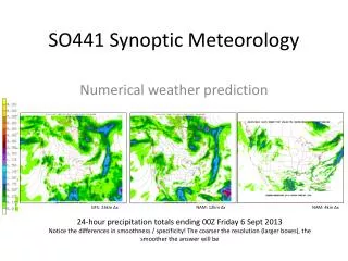
Analysis of weather observations • Observations includes: SYNOP observations, other observations(ex. automatic, flight and road weather observations soundings), satellite images, radar images, and observations from airplanes • A lot of observational data goes straight into the initial conditions of models. In particular, information from satellites is used to patch up the sparse network of oceanic observations. • SYNOP observations are analyzed. Analysis means: • visualizing the isolines of parameters • defining the areas where a given phenomenon may occur • identifying observational errors • achieving a clear interpretation of the data • An analysis will also suggest which numerical parameters are to be paid attention to!
Example: analyzing surface SYNOP observations • Isolinesof isobars • Surface pressure tendency isolines or isallobars • Local weather (areas with precipitation, fog/mist, thunder, showers, etc.) • Wind convergence zones • Isotherms • Other things (as required); wildfires, sizable dust clouds, etc. Low pressure center Secondary low center Low pressure trough High pressure center Secondary high center High pressure ridge Saddle point
An analyzed chart can be: • Working chart for oneself and colleagues such as Surface charts • Product for a customer such as • – Weather charts for magazines • – Briefing charts for aviation • – Ice and wind charts for shipping
Conceptual models: • simplified representations of the properties of weather systems • are not necessarily clear; weather systems are formed, die out, undergo change and are not always clear with regard to every parameter • vary according to surface, season and time of day • contain information about a system's development over time • There are manuals of conceptual models (SatManu, Lehkonen: käsitemallit), but interpreting the weather is subjective.
Why do we need manual analysis and interpretation? • Conceptual models cannot be identified automatically with existing equipment • One can spot errors in the model and anticipate developments that differ from the model’s predictions • Local conditions and factors relevant on the mesoscale can be taken into account (surface, season, history, etc.) • Humans can infer observational errors and the effects of sub-synoptic scale weather and environmental phenomena better than programs. • Drawing lines and conceptual models on a map improves one’s understanding of the issue at hand more than simply looking at finished products.
We need to understand these facts at the same temperature, air at a higher pressure is more dense than air at a lower pressure. at a given atmospheric pressure, air that is cold is more dense than air that is warm. it takes a shorter column of cold, more dense air to exert the same surface pressure as a taller column of warm, less dense air. Warm air aloft is normally associated with high atmospheric pressure, and cold air aloft is associated with low atmospheric pressure.
The relationship among the pressure, temperature, and density of air “referred to as the gas law (or equation of state)”, can be expressed by : Pressure = temperature × density × constant. When we ignore the constant and look at the gas law in symbolic form, it becomes where, p is pressure, T is temperature, and ρ represents air density. A change in one variable causes a corresponding change in the other two variables. 1. Suppose, we hold the temperature constant. The relationship then becomes: p ~ ρ (temperature constant) This expression says that the pressure of the gas is proportional to its density, as long as its temperature does not change. if the temperature of a gas (ex. air) is held constant, as the pressure increases the density increases, and vice versa. i.e, at the same temperature, air at a higher pressure is more dense than air at a lower pressure. In the atmosphere, with nearly the same temperature and elevation, air above a region of surface high pressure is more dense than air above a region of surface low pressure (see Fig.1).
We can see, then, that for surface high pressure areas (anticyclones) and surface low pressure areas (mid-latitude storms) to form, the air density (mass of air) above these systems must change. 2. What happens to the gas law when the pressure of a gas remains constant? the law becomes (Constant pressure) × constant = T ×ρ. ρ~ 1/T This relationship tells us that when the pressure of a gas is held constant, the gas becomes less dense as the temperature goes up, and more dense as the temperature goes down. Therefore, at a given atmospheric pressure, air that is cold is more dense than air that is warm. Keep in mind that the idea that cold air is more dense than warm air applies only when we compare volumes of air at the same level, where pressure changes are small in any horizontal direction.
To help eliminate some of the complexities of the atmosphere, scientists construct “ simple atmospheric model”, as shown in (figure 2) a column of air, extending well up into the atmosphere., the dots represent air molecules. Our model assumes: the air molecules are not crowded close to the surface and, unlike the real atmosphere, the air density remains constant from the surface up to the top of the column, the width of the column does not change with height. Suppose we somehow force more air into the column in Fig. 2. What would happen? • If the air temperature in the column does not change, the added air would make the column more dense, and the added mass of the air in the column would increase the surface air pressure. • Likewise, if a great deal of air were removed from the column, the surface air pressure would decrease.
Suppose the two air columns in Fig. 3a are located at the same elevation and have identical surface air pressures. This means that there must be the same number of molecules (same mass of air) in each column above both cities. • suppose that the surface air pressure for both cities remains the same, while the air above city 1 cools and the air above city 2 warms (see Fig. 3b). As the air in column 1 cools, the molecules move more slowly and crowd closer together—the air becomes more dense. In the warm air above city 2, the molecules move faster and spread farther apart—the air becomes less dense. • Since the width of the columns does not change, (and if we assume an invisible barrier exists between the columns), the surface pressure does not vary and the total number of molecules above each city must remain the same. Therefore, in the more dense cold air above city 1, the column shrinks, while the column rises in the less dense warm air above city 2.
We now have a cold shorter column of air above city 1 and a warm taller air column above city 2. From this situation, we can conclude that: • it takes a shorter column of cold, more dense air to exert the same surface pressure as a taller column of warm, less dense air. • This concept has a great deal of meteorological significance. • Atmospheric pressure decreases more rapidly with elevation in the cold column of air. In the cold air above city 1, move up the column and observe how quickly you pass through the densely packed molecules. This activity indicates a rapid change in pressure. • In the warmer, less dense air, the pressure does not decrease as rapidly with height, simply because you climb above fewer molecules in the same vertical distance. In Fig. 3c, move up the warm column until you come to the letter H. Now move up the cold column the same distance until you reach the letter L. Notice that there are more molecules above the letter H in the warm column than above the letter L in the cold column. The fact that the number of molecules above any level is a measure of the atmospheric pressure leads to an important concept:
Warm air aloft is normally associated with high atmospheric pressure, and cold air aloft is associated with low atmospheric pressure. In Fig. 3c, the horizontal difference in temperature creates a horizontal difference in pressure. The pressure difference establishes a force (called the pressure gradient force) that causes the air to move from higher pressure toward lower pressure. Consequently, if we remove the invisible barrier between the two columns and allow the air aloft to move horizontally, the air will move from column 2 toward column 1. As the air aloft leaves column 2, the mass of the air in the column decreases, and so does the surface air pressure. Meanwhile, the accumulation of air in column 1 causes the surface air pressure to increase. heating or cooling a column of air can establish horizontal variations in pressure that cause the air to move. The net accumulation of air above the surface causes the surface air pressure to rise, whereas a decrease in the amount of air above the surface causes the surface air pressure to fall.
Pressure at the bottom of each tank is a weight of water above; pressure at the bottom of A > pressure at the bottom of B; greater the difference higher the force
Pressure Gradient Force • Pressure Gradient = Pressure Difference/distance • Pressure Gradient Force is the force that causes the wind to blow; closely spaced isobars on a weather chart indicate steep pressure gradients, strong forces, and high winds • Pressure gradient force (PGF) is the Net force directed from higher toward lower pressure at right angles to the isobars • Magnitude of this force is directly related to the pressure gradient. • PGF between 1 & 2 is 4 mb/100km. Closer isobars--- greater pressure gradient--- stronger PGF--- greater the wind speed– length of arrows indicate magnitude of PGF
Pressure Systems Pressure varies from day-to-day at the Earth’s surface - the bottom of the atmosphere. This is, in part, because the Earth is not equally heated by the Sun. Areas where air is warmed often have lower pressure because the warm air rises and are called low pressure systems. Places where air pressure is high are called high pressure systems. Centers of surface high and low pressure areas are found within closed isobars on a surface weather analysis where there the absolute maxima and minima in the pressure field, and can tell a user in a glance what the general weather is in their vicinity and the wind is caused by air flowing from high pressure to low pressure its direction is influenced by the earth’s rotation. This is called pressure centers.
A low pressure system has lower pressure at its center than the areas around it. Winds blow towards the low pressure, and the air rises in the atmosphere where they meet. As the air rises, the water vapor within it condenses forming clouds and often precipitation too. Because of Earth’s spin and the Coriolis Effect, winds of a low pressure system swirl counterclockwise north of the equator and clockwise south of the equator. This is called cyclonic flow. On weather maps a low pressure system is labeled with red L, there are usually frontal systems associated with depressions. Low-pressure systems are associated withclouds andprecipitation that minimize temperature changes through the day
A high pressure system has higher pressure at its center than the areas around it. Wind blows away from high pressure. Winds of a high pressure system swirl clockwise north of the equator and counterclockwise south of the equator. This is called anticyclonic flow. Air from higher in the atmosphere sinks down to fill the space left as air blew outward and its compresses and warms as it descends, which inhibits the formation of cloud. On a weather map the location of a high pressure system is labeled with a blue H. high-pressure systems normally associated with dry weather and mostly clear skies with larger diurnal temperature changes due to greater radiation at night and greater sunshine during the day.
Is the location for these pressure systems the northern or the southern hemisphere?
Compare/Contrast Chart High and Low Pressure
Buys Ballot’s Law A rule in synoptic meteorology, announced in 1857 by Buys Ballot, of Utrecht, which states that if, in the northern hemisphere, one stands with one’s back to the wind, pressure is lower on one’s left hand than on one’s right, whilst in the southern hemisphere the converse is true. This law implies that, in the northern hemisphere, winds blow anticlockwise round a depression, and clockwise round an anticyclone; the converse is true in the southern hemisphere.
Contour Maps • Contour maps organize all the available data so we can make sense of it • Once contoured, you can determine wind direction, high and low pressure systems, locations of possible precipitation, fronts, regions of strong winds and changing temperatures --- ALL FROM A MAP! • It can show us : Regions of High and Low Pressure, Fronts, Temperature, Wind Direction and Speed, How your weather is going to change!
Types of contour lines • Isopleth is a line on a map that connects all the points of a given variable with the SAME SPECIFIED VALUE • Isobar - line of constant pressure • Isotherm - line of constant temperature • Isotach - line of constant wind speed • Isodrosotherm -a line of constant dew point • Isohyet -a line of constant precipitation accumulation • Isoneph -a line of constant cloudiness • Isohaline -a line of constant salinity (saltiness in the ocean) • Isoheight -a line of constant height • isotachs – lines of equal wind speed
There are a few rules when it comes to drawing contours. • Contours should never cross or touch . • Contours should be smooth; no corners (this isn’t dot-to-dot…contours should be a bit rounded) • Do not draw in any more details than the data allow (you should not draw dramatic curves where there is no station data to support this…also, you should not draw a 60 °F circle inside a 65 °F circle unless there is a station inside the circle with a temperature of less than 60 °F) • Contours should be closed or reach the edge of the map (do not start a line in the middle of the map or leave one hanging) • Contours should be labeled (don’t forget to write 60 °F on or at the end of the 60 °F contour)
Examples • Temperature observations • Where do we draw the 15°F isotherm????
Examples • Temperature observations • Where do we draw the 15°F isotherm????
Examples • Temperature observations • Where should we draw the 75ºF and 80ºF isotherms? • Where should we draw the 75F and 80F isotherms?
Examples • Temperature observations • Where should we draw the 75ºF and 80ºF isotherms? • Where should we draw the 75F and 80F isotherms?