Download
1 / 30
320 likes | 533 Vues
The Structure of the Continental Lithosphere:. Constraints from Receiver Functions Erin Cunningham - Grad Talks May 2014. Structure of Continental Lithosphere. The Continental Lithosphere – layer stable over 2.5 Ga

E N D
The Structure of the Continental Lithosphere: Constraints from Receiver Functions Erin Cunningham - Grad Talks May 2014
Structure of Continental Lithosphere • The Continental Lithosphere – layer stable over 2.5 Ga • From mantle xenoliths the base of the continental lithospheric mantle (CLM) ~200-250 km in depth • Seismic tomography suggests 200-250 km thick CLM • Converted seismic waves indicate low velocity discontinuity at 80-120 km globally within continents • Too shallow to be the base of the CLM • mid-lithospheric discontinuity (MLD) Lekic & RomanowiczEPSL 2011
Mid-lithospheric seismic discontinuity Though this 80-120 km is found globally – no clear explanation exists Chemical discontinuity MLD • Anisotropy – Chemical layer at MLD and base of CLM much deeper (Yuan and Romanowicz 2010) – North America • Seismic Tomography– Chemical MLD with Melt near solidus, slab accretion (Artemiva 2009) Other Discontinuity MLD • Ps Receiver Functions – Thermal Boundary at MLD and Chemical Boundary at base of CLM (Rychert and Shearer 2009) – Global • Seismic Reflection, Seismic Tomography, Magnetotelluircs – Chemical boundary with magmatic intrusions, presence of fluids , or phase transformation at at the MLD (Thybo 2006) – Global • Sp Receiver Functions – Remnants from slab accretion (Miller and Eaton 2010)- Canadian Shield
Guiding Questions • Is the MLD a single sharp discontinuity or a region where velocity changes gradually with depth? • Can we constrain how sharp or gradient the discontinuity is? • Ultimately, what is the origin of the MLD and what does it tell us about CLM formation ?
Goals • Improve converted wave techniques for noisy sediment dominated areas • Determine the gradient of the low velocity MLD from converted wave observations • Analyze converted waves for all available TA stations across the US • Map variations in MLD depth and gradient across the US
Receiver Functions Receiver Functions tell us about velocity contrasts in Earth’s structure Relative Velocity Structure Free Air Surface Time (S to P) Crust Lithosphere Lithosphere
Receiver Functions Receiver Functions tell us about velocity contrasts in earth’s structure Free Air Surface Time ( S to P ) Crust Lithosphere Lithosphere S wave
Receiver Functions Receiver Functions tell us about velocity contrasts in earth’s structure Free Air Surface Time (S to P) Crust Lithosphere Lithosphere S wave S wave
Receiver Functions Receiver Functions tell us about velocity contrasts in earth’s structure Free Air Surface Time (S to P) Crust Velocity Decrease with depth Lithosphere Lithosphere S wave S wave
Receiver Functions Receiver Functions tell us about velocity contrasts in earth’s structure Free Air Surface Time (S to P) Crust Velocity Increase with depth Lithosphere Lithosphere S wave S wave
Receiver Functions Receiver Functions tell us about velocity contrasts in earth’s structure Free Air Surface Time (S to P) Crust Lithosphere Lithosphere S wave S wave
Receiver Functions Receiver Functions tell us about velocity contrasts in earth’s structure Free Air Surface Time (S to P) Crust Lithosphere Lithosphere S wave S wave
Receiver Functions The Amplitude of the S to p conversion is due to the : • Sharpness of the Velocity change with depth • Total Change in Velocity Time ( S to P )
Sp Station Stacking Sp RFs are very noisy require stacking Sp RF have poor lateral resolution if stacked by station Map View – average depth for each station Free Air Surface v Crust v v Lithosphere v v Lithosphere S wave
Dense Seismic Arrays Earth scope USArray database – Enhance “pixels” of earth structure Prior Station Coverage
Common Conversion Point Stacking Map View – average depth all stations that sample the same area each station Sp Receiver Functions have better lateral resolution if stacked from all station Free Air Surface Crust Lithosphere Lithosphere S waves
Frequency Dependence of RFs • Consider a sharp vs a gradient velocity structure
Frequency Dependence of RFs • At low frequencies, seismic waves cannot “see” the difference between a sharp and gradational MLD
Frequency Dependence of RFs • At high frequencies, the gradational MLD produces weaker conversions
Sharp: Predicted Sp RFs Low Frequencies Medium Frequencies High Frequencies
Gradational: Predicted RFs Low Frequencies Medium Frequencies High Frequencies
Predicted Amplitude Ratio Moho to MLD (Positive to Negative)
Preliminary Results- Amplitude RatioMoho to MLD Data (F31A P01C) Station P01C – Willits, CA Station F31A – Hecla, SD
Preliminary Results- Amplitude RatioMoho to MLD Data (F31A P01C) Station P01C – Willits, CA Station F31A – Hecla, SD
Preliminary Results- Amplitude RatioMoho to MLD Data (F31A P01C) Station P01C – Willits, CA Station F31A – Hecla, SD
Guiding Questions • Is the MLD a single sharp discontinuity or a region where velocity changes gradually with depth? – the nature of the MLD seems to change with location. Age? Geologic structures? • Can we constrain how sharp or gradient the discontinuity is? – Yes, using the frequency dependence of gradient features. More work will be focused on quantifying the gradational structure • Ultimately, what is the origin of the MLD and what does it tell us about CLM formation ?
References Artemieva, I.M., (2006) Global 1°x1° model for the continental lithosphere: age, temperatures, and implications for lithosphere secular evolution. Tectonophysics 416, 245-277. C.A. H. Thybo, Tectonophysics416, 1-4 (2006) M.Miller, D.Eaton, Geophys. Res. Lett.37,18 (2010) Rychert, C.A, and Shearer, P.M., (2009) A Global View of the Lithosphere- Asthenosphere Boundary . Science. 324, 495-498. Yuan, H., and Romanowicz, B. (2010) Lithospheric Layering in the North American Craton. Nature. 466, 1063-1068.