Comparative Study on Effective Turbulence Model for NACA0012 Airfoil using Spalart – Allmaras as a Benchmark

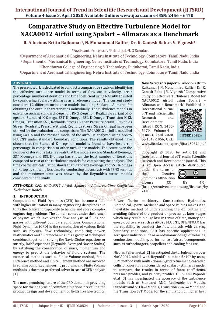
1. International Journal of Trend in Scientific Research and Development (IJTSRD) Volume 4 Issue 3, April 2020 Available Online: www.ijtsrd.com e-ISSN: 2456 – 6470 Comparative Study on Effective Turbulence Model for NACA0012 Airfoil using Spalart – Allmaras as a Benchmark R. Allocious Britto Rajkumar1, N. Mohammed Raffic2, Dr. K. Ganesh Babu3, V. Vignesh4 1,2Assistant Professor, 3Principal, 4UG Scholar, 1Department of Aeronautical Engineering, Nehru Institute of Technology, Coimbatore, Tamil Nadu, India 2Department of Mechanical Engineering, Nehru Institute of Technology, Coimbatore, Tamil Nadu, India 3Chendhuran College of Engineering & Technology, Pudukottai, Tamil Nadu, India 4Department of Aeronautical Engineering, Nehru Institute of Technology, Coimbatore, Tamil Nadu, India ABSTRACT The present work is dedicated to conduct a comparative study on identifying the effective turbulence model in terms of flow outlet velocity, error percentage, number of iterations and time coefficient using NACA0012 airfoil by considering Spalart – Allmaras as a reference model. The current study considers 12 different turbulence models including Spalart – Allmaras for obtaining the output characteristics individually. The turbulence models in existence such as Standard K-epsilon, RNG K-epsilon, Realizable variant of K- epsilon, Standard K-Omega, SST K-Omega, BSL K-Omega, Transition K-KL Omega, Transition SST, Reynolds Stress (Linear Pressure Strain), Reynolds Stress (Quadratic Pressure Strain), Reynolds stress (Stress Omega) have been utilized for the evaluation and comparison. The NACA0012 airfoil is modelled using CATIA and the meshed model of the airfoil is analyzed using ANSYS FLUENT under standard boundary conditions. The results obtained have shown that the Standard K – epsilon model is found to have less error percentage in comparison to other turbulence models. The count over the number of iterations taken reveals that the models such as Standard K-omega, SST K-omega and BSL K-omega has shown the least number of iterations compared to rest of the turbulence models for completing the analysis. The time coefficient calculation shows that Standard K-omega and SST K-omega ranks top by showing less time for conducting the analysis with 77.92 seconds and the maximum time was shown by the Reynolds’s stress models considered in the study. KEYWORDS: CFD, NACA0012 Airfoil, Spalart – Allmaras, Time Coefficient, Turbulence Models 1.INTRODUCTION Computational Fluid Dynamics (CFD) has become a field with higher utilization in many engineering disciplines due to its flexibility and capability to handle and solve complex engineering problems. The domain comes under the branch of physics which involves the flow analysis of fluids and gasses with different boundary conditions. Computational Fluid Dynamics (CFD) is the combination of various fields such as physics, flow technology, computing power, mathematics and fluid mechanics. It is a group of techniques combined together in solving the NavierStokes equations or strictly, RANS equations (Reynolds-Averaged Navier-Stokes) by satisfying the conservation of mass, momentum and energy to predict the behavior of fluidic systems. The numerical methods such as Finite Volume method, Finite Difference method and Finite Element method are involved in solving complex engineering problems and Finite Volume methods is the most preferred solver in case of CFD analysis [1]. The most promising nature of the CFD domain in providing space for the analysis of complex situations prevailing the product design and development of fields like Electronics, How to cite this paper: R. Allocious Britto Rajkumar | N. Mohammed Raffic | Dr. K. Ganesh Babu | V. Vignesh "Comparative Study on Effective Turbulence Model for NACA0012 Airfoil using Spalart – Allmaras as a Benchmark" Published in International Journal of Trend in Scientific Research and Development (ijtsrd), ISSN: 2456- 6470, Volume-4 | Issue-3, April 2020, pp.1049-1056, URL: www.ijtsrd.com/papers/ijtsrd30824.pdf Copyright © 2020 by author(s) and International Journal of Trend in Scientific Research and Development Journal. This is an Open Access article distributed under the terms of the Creative Commons Attribution License (CC (http://creativecommons.org/licenses/by /4.0) IJTSRD30824 BY 4.0) Power, Turbo machinery, Construction, Hydraulics, Biomedical, Sports, Medicine and Space studies makes it an inevitable method of understanding the difficulties and avoiding failure of the product or process at later stages which may result in huge loss in terms of time, money and energy. Software’s such as ANSYS FLUENT, OPENFOAM has the capability to conduct the flow analysis with varying boundary conditions. CFD has specific applications in aerospace industry such as aerodynamic design of vehicles, combustion modelling, performance of aircraft components such as turbochargers, propellers and cooling fans etc. Nicolas Pellerin et.al [2] investigated the turbulent flow over NACA0012 airfoil with Reynold’s number 5×105 by using LBM method with multi - domain grid refinement, cascaded collision operator and considered Spalart – Allmaras model to compare the results in terms of force coefficients, pressure profiles, and velocity profiles. Olubunmi Popoola et.al [3] has investigated the accuracy of the turbulence models such as Standard, RNG, Realizable k-ɛ Models, Standard and SST k-ω Models, Transition k -kL-ω Model and the Transition SST Model for the simulation of higher heat @ IJTSRD | Unique Paper ID – IJTSRD30824 | Volume – 4 | Issue – 3 | March-April 2020 Page 1049

2. International Journal of Trend in Scientific Research and Development (IJTSRD) @ www.ijtsrd.com eISSN: 2456-6470 transfer rate for Reciprocating Mechanism Drive Heat Loop device by using CFD solver and they have found that the Standard k-ɛ Models provides the least prediction and the RNG k-ɛ Models has higher accuracy than all other models. Manuel Garcia Pérez, Esa Vakkilainen [4] has made a comparison on the turbulence models such as URANS k-ɛ and DES and the two and three dimensional mesh approaches in terms of their capability of providing highly accurate results and computational cost by considering the unsteady CFD ash deposition tools. A. Riccia et.al [5] has investigated the impact of the turbulence model and roughness height selection 3D steady RANS simulations of wind flow in an urban environment and they have found that the turbulence models have more impact comparing to the surface roughness parameters considered. Abdolrahim et.al [6] has conducted a study to understand the accuracy of the turbulence models for CFD simulations of vertical axis wind turbines using the one equation and two equation models with an additional intermittency transition model (SSTI) models. The authors have reported that models such as SA, RNG, Realizable k-ε and k-kl-u models failed to reproduce the aerodynamic performance of VAWTs. The variables of SST model is found to have good agreement with the experimental data sets than other models. Tao Zhi et.al [7] has studied the effect of turbulence models in predicting the convective heat transfer to hydrocarbon fuel at supercritical pressure and found that SST model and Launder and Sharma model performed well compared to other models. Mohamed M.Helal et.al [8] studied the numerical simulation of cavitation flow over marine propeller blades using transition –sensitive turbulence model in comparison with the standard K-epsilon model and they have found that the prediction based upon k-kl-ω transition model has good agreement with the experimental data set. V.K.Kratsev et.al [9] has reviewed the role of URANS and LES hybrid simulations in the field of internal combustion engine application for the development and optimization. Feng Gao et.al [10] attempted to compare the different turbulence models in simulating unsteady flow and they have found that robustness of the standard turbulence models are superior to low Reynolds’s model. M. Ghafari and M.B. Ghofrani [11] has studied about the effects of overestimation or underestimation of turbulence characteristics at the interface by using a new turbulence model. Jia-Wei Han et.al [12] conducted a study on various CFD turbulence models on for refrigerated transport of fresh fruit and found that SST k- ω models have shown agreement with measured experimental data set. Aoshuang Ding et.al [13] has conducted numerical investigation of turbulence models for a superlaminar journal bearing by considering 14 different turbulence models and concluded that the SST model with low –re number yields the best results in comparison. Douvi C. Eleni et.al [14] has compared the various turbulence models for the NACA0012 airfoil for a two dimensional subsonic flow at various angles of attack and Reynolds’s number 3 x 106 and highlighted that the areas transition model prediction and turbulence modelling requires further investigation as no model is found to be providing more accurate results at higher FernandoVillalpando et.al [15] assessed the flow simulation of different turbulence models for the wind turbine airfoil of NACA 63-415 model at various angles of attack by using the one equation and two equation models available in commercial packages. The authors have concluded that SA model is good in predictions of near maximal lift and the SST k-ω model is the best turbulence model for simulating flow around both clean and iced wind turbine airfoils. 2.Turbulence Models The current sections explains about the various turbulence models present in the study for conducting the flow simulations In total the study considers 12 different turbulence models which are in existence and from that the model Spalart-Allmaras has been considered as a standard for comparison. Turbulence flow modelling through computational software has an objective to predict the quantities of interest such as fluid velocity, pressure and other related characteristics. Turbulence models can be classified based upon the computational cost, finer the resolution of the simulation, length of the turbulent scales, accuracy. 2.1.Spalart – Allmaras From the day of its introduction on 1992, this model is found to have more application in the field of aerodynamics in solving problems with turbulent flow. This method is considered to be the most efficient and effective model for conducting the aerodynamic flow analysis in structures such as airfoils, wings, fuselages, missiles and ship hulls by the simulation community as it takes lesser time, iterations and cost to provide results of higher accuracy [16] . This one – equation turbulence models is used in aerospace applications with wall bounded flows and it has shown appreciable results for problems with boundary layers subjected to adverse pressure gradients. This method has obvious applications in the field of turbo machinery due to its potential to provide results with higher accuracy. 2.2.Standard K-ε Model A two equation model which gives a general description of turbulent flows by means of two transport equation in the form of PDE’s. The model has more utilization in CFD softwares for the simulation of turbulent flows at varying boundary conditions. The transport equations are not in integration to the walls but the factors such as production and dissipation of kinetic energy are well specified in the near wall using the wall’s logarithmic law. 2.3.RNG K-ε Model Renormalization Group K-ε model is a mathematical technique which results in the modified form of standard K-ε model to make an attempt for the different scales of motion through changes to production term. The standard model considers only the single turbulence length scale to determine the eddy viscosity but in reality all scales of motion will contribute to the turbulent diffusion characteristics of the flow. 2.4.Realizable variant of K-ε Model The term realizable represents the nature of the model in satisfying certain mathematical constraints over the parameter Reynolds’s Stress which are in consistent with the physics of the turbulent model. It is an improvement over the standard K-ε Model and differs from the same in two different ways. The developed. K-ε Model consists a new formulation for theturbulent viscosity and a new transport equation for the dissipation rate ɛ. For flows with an involvement of rotation, boundary layers under strong adverse pressure gradients, separation, and recirculation can be solved with this model with an achievement of superior angle of attack. @ IJTSRD | Unique Paper ID – IJTSRD30824 | Volume – 4 | Issue – 3 | March-April 2020 Page 1050

3. International Journal of Trend in Scientific Research and Development (IJTSRD) @ www.ijtsrd.com eISSN: 2456-6470 performance. The model also demonstrates a superior capability in capturing the mean flow around complex structures involved in the analysis. 2.5.Standard K-Omega The model with two equations which generally attempts to predict turbulence by two PDE for the two variables namely turbulence kinetic energy (K) and Specific rate of dissipation (ω). The model is a two equation turbulence model which has a very high closeness with RANS (Reynold’s Averaged Navier – Stokes) equations. 2.6.SST K-omega The Shear Stress Transport (SST) in combination with K- omega is a two equation eddy viscosity model which has gained more popularity due to its flexibility in solving the turbulent flow problems involving low Reynolds’s number. The model is recommended by many users for its meritorious good behaviour in the separating flow and adverse pressure gradients. The model has a tendency to produce a too large turbulence levels in regions with strong acceleration which is actually less pronounced with normal K-ε Model. 2.7.BSL K-omega The Baseline (BSL) model with Bradshaw’s assumption with two equations designed to provide results similar to that of real K-Omega model of Wilcox and it has an identity of around 50% of the boundary layer with gradual changes. The results obtained by this model is similar in nature with respect to K-omega model with som exceptions. 2.8.Transition K-KL omega A newly developed three equation model which actually applicable for incompressible flows with a low Reynold’s number. It actually applied towards the transition of a flow from laminar to turbulence. The model has equations for laminar kinetic energy, turbulent kinetic energy and specific dissipation rate. The model can be simulated using OPENFOAM software. 2.9.Transition SST The model is primarily applicable to only wall bounded flows which is not a Galilean invariant and it cannot be applied for transition in free shear flows. The model is not suitable for wall jet flows. The model is designed for flows with a defined nonzero freestream velocity. 2.10.Reynolds stress (Linear Pressure Strain) The Reynold’s Stress model which considers the pressure strain term in three different categories namely slow pressure –strain term, rapid pressure – strain term and wall reflection term with equations by including the pressure strain term as default one. The same model when applied to near-wall flows described with two layer model requires the modification of pressure strain term. 2.11.Reynolds stress (Quadratic Pressure Strain) The model is considered as an optional pressure – strain model proposed by Speziale, Sarkar, and Gatski. The model provides high performance in a range of basic shear flows, plane strain, rotating plane shear and axisymmetric expansion / contraction. The model provides enhanced accuracy for flows with more complexity in particular with streamline curvature. 2.12.Reynolds stress (Stress Omega) The stress transport model based upon omega equations and LRR model which finds applications in modelling flows with curved surfaces and swirling flows. The model resembles the K-Omega model in terms of prediction capacity for a wide range of turbulent flows. The model can be selected from the viscous model dialog box in ANSYS FLUENT. 3.Modeling and Analysis The present work considers the NACA0012 (National Advisory Committee for Aeronautics) airfoil for conducting the analysis and the 3D model of the airfoil is created using CATIAV5R20 software with a total of 164 coordinate points. The airfoil has a chord length of 100mm with a thickness of 10mm.The airfoil is modelled using simple 2D commands such as spline, mirror, connect curve and join in the sketcher module and pad command is used for converting the 2D sketch in to 3D model of the airfoil section. The Figure No 3.1 shows the 3D model of the NACA0012 airfoil. Fig No 3.1 NACA0012 Airfoil 3D Model The 3D model of the airfoil created using CATIAV5R20 software is saved in the .igs format and imported to ANSYS analysis package for further analysis of turbulent models. The airfoil is considered to behave like a cantilever beam.The geometry section and airfoil is meshed in the ANSYS workbench with a maximum of 3, 00,000 elements and 54,548 nodes connecting the elements by adopting fine quality mesh which is generally considered to achieve results with higher accuracy. The meshed geometry is further exported to FLUENT module for conducting the analysis. The inlet flow is created and made to flow over the airfoil section and the output velocity of all the models are tabulated to comparison. Fig No 3.1 Meshed View of the Enclosure Fig No 3.2 Meshed View of NACA0012 Airfoil @ IJTSRD | Unique Paper ID – IJTSRD30824 | Volume – 4 | Issue – 3 | March-April 2020 Page 1051

4. International Journal of Trend in Scientific Research and Development (IJTSRD) @ www.ijtsrd.com eISSN: 2456-6470 The Table No 3.1 shows the NACA0012 Airfoil Dimensions and Inlet Flow Properties considered in the present study. Table No 3.1 NACA0012 Airfoil Dimensions and Inlet Flow Properties S. No Parameters / Characteristics Symbol S.I Unit 1 Length 2 Thickness 3 Reynold’s Number 4 Pressure 5 Velocity 6 Turbulent Intensity 7 Turbulent Kinetic Energy 8 Turbulent Length Scale 9 Turbulent Dissipation Rate 10 Specific rate of dissipation 11 Turbulent viscosity ratio 4.Results and Discussion The flow simulations obtained for the various turbulence models have been noted for its value towards the output characteristic velocity of the flow after flowing over the NACA0012 airfoil and the values are tabulated in terms of both velocity contour and velocity vector. The one equation Spalart Allmaaras model is considered to be the standard model for comparison with other 11 different turbulence models considered. The error coefficient value obtained with respect to the standard model for other turbulence models and the number of iterations occurred for the individual turbulence model and time coefficient is also compared. The Table No 4.2 shows the results obtained for various turbulence models such as error coefficient, number of iterations and time coefficient through flow analysis using ANSYS FLUENT module. Table No 4.1 Results of Various Turbulence Models for Velocity in terms of Contour and Vector Value 100 10 507596.685 101325 75 3.06 8.09233848 0.007 5.40374578×102 6004.16188 738.164555 l t mm mm NA Pascal m/s % m2/s2 m Re P v I k L ? ? ?? / ? m2/s2 1/s NA Velocity (m/s) Contour 8.881×101 8.971×101 8.896×101 8.986×101 8.923×101 9.013×101 8.911×101 9.002×101 8.923×101 9.014×101 8.923×101 9.013×101 8.897×101 8.987×101 8.980×101 9.071×101 8.910×101 9.000×101 8.937×101 9.027×101 S. No Turbulence Models Vector 1 2 3 4 5 6 7 8 9 10 11 12 Spalart-Allmaras Standard K-epsilon RNG K-epsilon Realizable variant of K-epsilon Standard K-Omega SST K-Omega BSL K-Omega Transition K-KL mega Transition SST Reynolds Stress (Linear Pressure Strain) Reynolds Stress (Quadratic Pressure Strain) 8.932×101 9.023×101 Reynolds stress (Stress Omega) 8.900×101 8.990×101 The tabulated output velocity in terms of contour and vector are further used for calculating the error percentage that exists between the velocity value of the standard turbulence model and other models considered for study. A total of 24 simulations has been generated through FLUENT solver for both the velocity contour and vector of all the turbulence models considered. The outlet flow velocity has been calculated for all the turbulence models considered and the values of velocity has been recorded in terms of both contour and vector form and tabulated for further analysis and comparison. From the simulation results the outlet velocity obtained for Spalart Allmaras model is found to be 8.881×101 m/s in contour form and 8.971×101 m/s in vector form. The outlet values velocity obtained of other turbulence model is found to the higher in case of both the contour and vector forms for all the turbulence models. The lowest outlet velocity values in terms of both contour and vector form is obtained for Standard K –epsilon model (8.896×101 m/s and 8.986×101 m/s) and the highest outlet velocity values in terms of both contour and vector form is obtained for the Transition K-KL omega model with 8.980×101 m/s and 9.071×101 m/s respectively. The outlet velocity values obtained for RNG K-epsilon, Standard K – Omega and SST K-omega in contour form is found to be similar (8.923×101 m/s). The simulation of velocity in contour and vector form for the standard Spalart – Allmaras model has been shown in Fig No 4.1 and 4.2. The sample of few CFD simulations of turbulence models with less error percentage, less number of iterations for completing the analysis and less time coefficient are shown in Fig No 4.3, 4.4, 4.5, 4.6, 4.7, 4.8 for reference. @ IJTSRD | Unique Paper ID – IJTSRD30824 | Volume – 4 | Issue – 3 | March-April 2020 Page 1052

5. International Journal of Trend in Scientific Research and Development (IJTSRD) @ www.ijtsrd.com eISSN: 2456-6470 Fig No 4.3 Contour View of Spalart – Allmaras Model Fig No 4.4 Vector View of Spalart – Allmaras Model Fig No 4.5 Contour View of Standard K-epsilon Model @ IJTSRD | Unique Paper ID – IJTSRD30824 | Volume – 4 | Issue – 3 | March-April 2020 Page 1053

6. International Journal of Trend in Scientific Research and Development (IJTSRD) @ www.ijtsrd.com eISSN: 2456-6470 Fig No 4.6 Vector View of Standard K-epsilon Model Fig No 4.7 Contour View of Standard K-omega model Fig No 4.8 Vector View of Standard K-omega model @ IJTSRD | Unique Paper ID – IJTSRD30824 | Volume – 4 | Issue – 3 | March-April 2020 Page 1054

7. International Journal of Trend in Scientific Research and Development (IJTSRD) @ www.ijtsrd.com eISSN: 2456-6470 Table No 4.2 Results of Various Turbulence Models for Error Coefficient, Number of Iterations and Time Coefficient Error Percentage Contour 1 Spalart-Allmaras 2 Standard K-epsilon 0.1686 3 RNG K-epsilon 0.4729 4 Realizable variant of K-epsilon 0.3366 5 Standard K-Omega 0.4729 6 SST K-Omega 0.4729 7 BSL K-Omega 0.1801 8 Transition K-KL Omega 1.1024 9 Transition SST 0.3265 10 Reynolds Stress (Linear Pressure Strain) 0.6305 11 Reynolds Stress (Quadratic Pressure Strain) 0.5742 12 Reynolds stress (Stress Omega) 0.2139 Number of Iterations 30 43 43 43 39 39 39 94 48 121 236 221 S. No Turbulence Models Time Coefficient (s) Vector 0 0.1669 0.4659 0.3455 0.4793 0.4659 0.1783 1.114 0.3232 0.6240 0.5796 0.2117 0 59.4 128.87 85.91 85.91 77.92 77.92 119.1 281.71 143.85 487.51 707.29 883.11 Conclusion The Following points may be used for concluding the present work conducted through ANSYS simulation software. 1.The most adopted Spalart-Allmaras turbulence model in case of aerodynamics flow analysis has been taken as the standard reference turbulence model for comparison with the other 11 different turbulence models considered for studying the flow analysis of NACA0012 airfoil 2.In the estimation of error percentage, Standard K – epsilon model is found to have less error percentage in comparison to other turbulence models. The turbulence models such as Transition K-KL omega, Reynolds stress (Linear pressure strain) and Reynolds stress (Quadratic pressure strain) have shown higher error percentage. 3.The number of iterations occurred for the turbulence model has been considered as one of the output characteristic and compared with each other. The models such as Standard K-omega, SST K-omega and BSL K-omega has used less number of iterations in comparison with other turbulence models. 4.The maximum iterations were shown by Reynolds stress (Quadratic pressure strain) model with 236 iterations followed by Reynolds stress (Stress omega) with 221 iterations and Reynolds stress (Linear pressure strain) with 121 iterations when compared to the standard turbulence model with 30 iterations. 5.The number of iterations taken by the Reynolds stress (Quadratic pressure strain) model, Reynolds stress (Stress omega) and Reynolds stress (Linear pressure strain) are found to be taking 8 times, 7.5 times and 4 times more than the standard model. 6.The models such as Standard K-omega, SST K-omega and BSL K-omega has shown only 39 number of iterations which is slightly higher than the Spalart Allmaras model with 30 iterations. 7.The other models such as Standard K-epsilon, RNG K- epsilon and Realizable variant of k-epsilon has shown 43 iterations and found similar with each other. 8.In case of time coefficient calculation, the models such as Standard K-omega and SST K-omega have shown less time for conducting the analysis with 77.92 seconds and ranks top when compared to the Spalart-Allmaras turbulence model with 59 seconds. The time taken by both the models are found to be 32 % higher than the standard model. The number of iterations for both the models are found to be same. 9.Next to the top ranking models in low time coefficient the models such as RNG K-epsilon, Realizable variant of k-epsilon have shown 85.91 seconds and it is found to be 45.61 % more time than the standard model. 10.The other considered models such as BSL K-omega, Standard K-epsilon and Transition SST have shown time coefficient values of 119.106 seconds, 128.871 seconds and 143.856 seconds respectively which are found to be more time consuming than standard models in the order of 102 %, 118.42 % and 144 % respectively. 11.The maximum time coefficient was obtained for Reynolds stress (Stress omega) model with 883.11 seconds followed by Reynolds stress (Quadratic pressure strain) with 707.29 seconds and Reynolds stress (Linear pressure strain) with 487.51 seconds when compared to the standard model with 59.4 seconds. 12.In comparison with standard turbulence model the maximum time coefficient obtained for models such as Reynolds stress (Stress omega), Reynolds stress (Quadratic pressure strain) and Reynolds stress (Linear pressure strain) are found to be more time consuming in the order of 1396 %, 1098% and 726.28% respectively. 13.The more time consuming models such as Reynolds stress (Quadratic pressure strain) and Reynolds stress (Linear pressure strain) are taking more number of iterations with higher time and error percentage may be avoided in conducting turbulence model analysis. The Reynolds stress (Stress omega) model is also showing higher time coefficient and iterations but in case of error percentage it is found to be less than other Reynolds stress models. 14.From the current study of flow analysis over an airfoil at subsonic conditions Spalart Allmaras is found to be the better one in providing accurate results than other turbulence models. REFERENCES [1]Ram Kumar Raman, Yogesh Dewang Jitendra Rag, “A review on applications of computational fluid dynamics “, International Journal of LNCT, 2018, Vol 2(6). [2]Nicolas Pellerin, Sébastien Leclaire, Marcelo Reggio, “An implementation turbulence model in a multi-domain lattice Boltzmann method for solving turbulent airfoil flows”, 2015, Computers and Mathematics with Applications, Vol 70, 3001–3018. of the Spalart–Allmaras @ IJTSRD | Unique Paper ID – IJTSRD30824 | Volume – 4 | Issue – 3 | March-April 2020 Page 1055

8. International Journal of Trend in Scientific Research and Development (IJTSRD) @ www.ijtsrd.com eISSN: 2456-6470 [3]Olubunmi Popoola, YidingCao, “ The influence of turbulence models on the accuracy of CFD analysis of a reciprocating mechanism driven heat loop “. Case Studies in Thermal Engineering (2016), Vol 8, pp 277– 290. Internal Combustion Engines simulation, Energy Procedia, 2018, Vol 248, 1098 – 1104. [10]Feng Gao, Haidong Wanga, Hui Wang, “Comparison of different turbulence models in simulating unsteady flow”, Procedia Engineering 205 (2017) 3970–3977. [4]Manuel García Pérez?, Esa Vakkilainen, “A comparison of turbulence models and two and three dimensional meshes for unsteady CFD ash deposition tools” ,2019, Fuel 237, pp 806-811. [11]M. Ghafari, M. B. Ghofrani, “New Turbulence modeling for air/water Stratified flow“, Journal of Ocean Engineering and Science, 2020, Vol 5, pp 55- 67. [12]Jia-Wei Han, Wen-Ying Zhu, Zeng-Tao Ji, “Comparison of veracity and application of different CFD turbulence models for refrigerated Intelligence in agriculture, 2019, Vol 3 pp 11 -17. [5]A. Riccia,b,c,, I. Kalkmanb, B. Blockena,, M. Burlandoc, M.P. Repettoc, “Impact of turbulence models and roughness height in 3D steady RANS simulations of wind flow in an urban environment”, 2020, Building and Environment, Vol 17. transport“, Artificial [13]AoshuangDing, XiaodongRen, XuesongLi ,ChunweiGu, “Numerical Investigation of Turbulence Models for a Superlaminar Journal Bearing “, Advances in tribology, 2018 . [6]Abdolrahim Rezaeiha, Hamid Montazeri, Bert Blocken, “On the accuracy of turbulence models for CFD simulations of vertical axis wind turbines “, 2019, Energy, Vol 180, pp 838 – 857. [14]Douvi C. Eleni, Tsavalos I. Athanasios Margaris P. Dionissios, “Evaluation of the turbulence models for the simulation of the flow over a National Advisory Committee for Aeronautics (NACA) 0012 airfoil “, Journal of Mechanical Engineering Research, 2012, Vol 43, pp 100 -111. [7]Tao Zhi, Cheng Zeyuan, Zhu Jianqin, Li Haiwang, “ Effect of Turbulence models on predicting convective heat transfer to hydrocarbon fuel at supercritical pressure “, 2016, Chinese Journal of Aeronautics, pp 1247 – 1261. [8]Mohamed M. Helal, Tamer M. Ahmed, Adel A. Banawan, Mohamed A. Kotb, “Numerical prediction of sheet cavitation on marine propellers using CFD simulation with transition sensitive turbulence model”, 2018, Alexandria Engineering Journal, Vol 57, 3805 – 3815. [15]FernandoVillalpando, Marcelo Reggio, AdrianIlinca, “Assessment of Turbulence Models for Flow Simulation around a Wind Turbine Airfoil”, Modelling and Simulation in Engineering, 2011. [16]ANSYS Customer Training Manual, “Turbulence Modeling”, Introductiion to ANSYS FLUENT. [9] V. K. Krastev, G. Di Ilio, G. Falcucci G. Bella, “ Notes on the hybrid URANS/LES turbulence modelling for @ IJTSRD | Unique Paper ID – IJTSRD30824 | Volume – 4 | Issue – 3 | March-April 2020 Page 1056