Download
1 / 137
1.4k likes | 1.65k Vues
Graphs and Graph Theory in Computational Biology. Dan Gusfield Miami University, May 15, 2008 (four hour tutorial) . Some examples of graphs in biology. Taken from the web - see the citations for details. Many other examples of graphs more complex than trees in biology.

E N D
Graphs and Graph Theory in Computational Biology Dan Gusfield Miami University, May 15, 2008 (four hour tutorial)
Some examples of graphs in biology • Taken from the web - see the citations for details. Many other examples of graphs more complex than trees in biology.
Yeast protein interactions From http://www-personal.umich.edu/~mejn/networks/
Protein-Protein Interaction Modelling Dr. Peter Uetz Institut fur Toxikologie und Genetik Forschungszentrum Karlsruhe
NY Times May 5, 2008 The Diseasome http://www.nytimes.com/interactive/2008/05/05/science/20080506_DISEASE.html
Graphs and Graph Theory 1. Numerous uses of graphs and networks to represent biological phenomena at many conceptual levels. Maybe several 1000s of papers using graph representations, particularly trees, but little graph theory. 2. A respectable number of papers that develop new non-trivial graph theory for problems in biology. 100s of papers, maybe 1000. 3. A handful of papers exploiting or extending non-trivial classic graph theory for problems in biology. Perhaps a few hundred.
Introduction and Conclusion Very diverse biological applications and very diverse graph theory. So no single grand reason for graphs and no single graph topic in biology. Lots of opportunity for graph theorists and graph algorithmists to develop or apply graph theory to biological problems. Even more opportunity for combinatorial optimization.
What I will do in this tutorial • Emphasis on points 2 and 3, i.e., Examples of the development of new non-trivial graph theory, and of the exploitation of classic graph theory. And (my apologies) I will mostly emphasize topics I have been involved with. Still, • There are some hot biological areas today where graphs arise, and some graph topics that recur commonly, and I should point those out even if I will not talk in detail on those topics.
The digression • Hot biology: Network biology -- biological phenomena that are represented by networks -- gene regulatory networks and protein interaction networks, just to name two. These form the core of Systems biology. Other relationships in biology represented by graphs and networks. Ex. diseasome. • Recurring graph problems: graph problems in clustering data ( ex. finding cliques or variants of cliques); variants of graph isomorphism in network motif or molecular pathway problems; need for more random graph theory for significance testing
Clique Problems Clique problems are recurrent in clustering applications, but true cliques are computationally hard to find. Suggested research for graph theorist and algorithmists: computationally tractable, biologically meaningful alternatives to cliques. As examples: maximum density subgraphs; extreme sets in a graph.
Subgraph density • Given a graph G, and a subset S of its nodes, let G(S) be the subgraph of G induced by S, i.e, G(S) has node set S and edge set E(S) consisting of all edges in G both of whose ends are in S. • A Maximum Density subgraph of G is induced by the set of nodes S which the Maximizes |E(S)|/|S|. • The maximum density subgraph can be found in polynomial time. It has the flavor of a maximum clique, but has different properties.
Extreme Sets In an edge-weighted undirected graph G, a subset S of nodes of G is called an extreme set if for every subset S’ of S, the total weight of the edges crossing from S’ to V-S’ is larger than the total weight of the edges crossing from S to V-S. All the extreme sets in a graph can be found in polynomial time.
Also There is also a great need for more sophisticated application of random graph theory in the study of biological networks. This is needed in order to establish null models to use in assessing the statistical significance of subgraphs, paths, patterns and motifs that are found in biological networks. We need to be able to distinguish observed patterns and subgraphs from those that occur with a high probability in a random graph, under a biologically appropriate model of randomness (an open field).
End of digression Start of the main tutorial: Examples of Graph Theory in Bioinformatics and Computational Biology
Outline • Three Smaller examples: Euler paths and sequencing; Tanglegrams and co-evolution; Network Design and Multiple Alignment. • Haplotyping by Perfect Phylogeny: Graph Realization. • Phylogenetic Networks: Incompatibility Graph; Galled-Trees; Recombination Networks; The Decomposition Theorem and sufficient conditions. • Multi-state Perfect Phylogeny and Chordal Graphs.
To start: Three small examples • Euler paths in sequencing and sequence assembly. • Tanglegrams and planarity testing in the study of co-evolution. • Application of Tree-Design approximations in multiple sequence alignment. Interplay between trees and strings.
Topic I: Eulerian paths in sequencing problems The general situation is that we have a (DNA say) molecule S whose sequence is unknown, but we know all the k-mers that occur in S, for some fixed k. Given those k-mers, we want to determine S, if possible, or determine whatever is possible to determine about S. Note that k is not related to the alphabet size. A very useful approach to problems of this type is to build an Eulerian digraph, based on the (k-1)-mers.
Euler graph for general k For general k, there is one node for each (k-1)-mer contained in an observed k-mer. Then there is a directed edge from the node for (k-1)mer A to the node for (k-1)mer B, if the (k-2) suffix of A matches the (k-2) prefix of B, so that A and B can be overlapped to form the observed k-mer. Example: k = 5 and we observe the 5-mer XXYZW. Then there will be a node for XXYZ and a node for XYZW and a directed edge from the first node to the second node. Those two nodes and the directed edge between them represent the 5-mer XXYZW. In some applications, there will be one such edge for each observation of that 5-mer.
Ex. k = 3. The graph will have one node for each of the 2-mers in the observed 3-mers. Then there is a directed edge from the node for the 2-mer XY to the node for the 2-mer YZ, for any X, Z. The Euler graph derived from the sequence ACACGCAACTTAAA If a triple is observed more than once, there should be One directed edge for each observation of the triple.
The point: Every Eulerian path in the graph specifies a sequence whose k-mers match the given data, and conversely every sequence whose k-mers match the data specifies an Eulerian path in the graph. So the set of Eulerian paths specifies the set of candidate sequences for the unknown original sequence. Algorithms exist for efficiently finding Eulerian paths, for counting their number, for determining uniqueness etc. so we can use this representation to study the set of candidate sequences. Compare this approach to earlier efforts to represent the set of candidates by a graph with a Hamilton path: each node represents an observed k-mer, not a (k-1)-mer.
Making finer distinctions in Euler paths In general there may be many Eulerian paths in the graph, and we want some additional criteria to distinguish the goodness of one Eulierian path compared to another. Different biological considerations translate into having a value for each subpath of length two. Then the value of an Eulerian path P with n edges is the sum of the n-1 values of the n-1 length-two subpaths in P. The problem is to find an Eulerian path with maximum value. We have some reasonable approximations for that, but a simpler case can be solved optimally in polynomial time.
The case of a binary alphabet, but arbitrary k Since the alphabet size is two, each node in the graph has at most two incoming edges and two outgoing edges. Assume exactly two each. 001 110 Ex. k = 4 011 110 101
The case of a binary alphabet, but arbitrary k At any node, there are two possible ways for an Euler path to pass through the node. 001 110 turning Ex. k = 4 011 110 101
The case of a binary alphabet, but arbitrary k At any node, there are two possible ways for an Euler path to pass through the node. 001 110 crossing Ex. k = 4 011 110 101 So in terms of subpaths of length two, we have two choices at each node.
Restating the optimal Euler path problem We are given an Eulerian graph where the in and out degrees are at most two at each node, and at each node there is a given value for the turning pair, and a value for the crossing pair. Then choose the turning or the crossing pairs at the nodes to maximize the total value of the choices, subject to the requirement that the choices create an Euler path in the graph.
Main Result • The problem can be solved in polynomial time. • The set of choices that give Euler paths has a matroidal structure, which allows a matroid-greedy algorithm to find the optimal Euler path. • A more direct algorithm based on Minimum Spanning Trees also solves the problem.
The Matroid Structure • At every node v, the edge pair (crossing or turning) which has the lowest value is called the low pair, and the other pair is the high pair. The difference in values is called the loss at v. • A subset S of nodes is called independent if there is an Euler path in the graph where at every node in S, the low pair is chosen. • As defined, the family of independent sets form a matroid, and so we can find, by a greedy algorithm, an independent set which minimizes the loss - and this gives the optimal Euler path.
Topic II: Tanglegrams • A Tanglegram is a pair of trees drawn in the plane with no crossing edges, with the same labeled leaf set. The leaves of one tree are displayed on a line, and the leaves of the other tree are displayed on a parallel line. • A straight line connect each leaf in one tree to the leaf with the same label in the other tree. • The number of crossing lines is a measure of the similarity of the trees.
Topic III: Multiple Sequence Alignment Interplay between sequences and trees. Exploitation of network design approximation.
Intro to Hours 2 and 3: Two “Post-HGP” Topics Two topics in Population Genomics • SNP Haplotyping in populations • Reconstructing a history of recombination These topics in Population Genomics illustrate current challenges in biology, and illustrate the use of graph theory, combinatorial algorithms and discrete mathematics in biology.
What is population genomics? • The Human genome “sequence” is done. • Now we want to sequence many individuals in a population to correlate similarities and differences in their sequences with genetic traits (e.g. disease or disease susceptibility). • Presently, we can’t sequence large numbers of individuals, but we can sample the sequences at SNP sites.
SNP Data • A SNP is a Single Nucleotide Polymorphism - a site in the genome where two different nucleotides appear with sufficient frequency in the population (say each with 5% frequency or more). • SNP maps have been compiled with a density of about 1 site per 1000. • SNP data is what is mostly collected in populations - it is much cheaper to collect than full sequence data, and focuses on variation in the population, which is what is of interest.
Haplotype Map Project: HAPMAP • NIH lead project ($100M) to find common SNP haplotypes (“SNP sequences”) in the Human population. • Association mapping: HAPMAP used to try to associate genetic-influenced diseases with specific SNP haplotypes, to either find causal haplotypes, or to find the region near causal mutations. • The key to the logic of Association mapping is historical recombination in populations. Nature has done the experiments, now we try to make sense of the results.
Topic IV: Perfect Phylogeny Haplotyping via Graph Realization
Genotypes and Haplotypes Each individual has two “copies” of each chromosome. At each site, each chromosome has one of two alleles (states) denoted by 0 and 1 (motivated by SNPs) 0 1 1 1 0 0 1 1 0 1 1 0 1 0 0 1 0 0 Two haplotypes per individual Merge the haplotypes 2 1 2 1 0 0 1 2 0 Genotype for the individual
Haplotyping Problem • Biological Problem: For disease association studies, haplotype data is more valuable than genotype data, but haplotype data is hard to collect. Genotype data is easy to collect. • Computational Problem: Given a set of n genotypes, determine the original set of n haplotypepairs that generated the n genotypes. This is hopeless without a genetic model.
The Perfect Phylogeny Model for SNP sequences Only one mutation per site allowed. sites 12345 Ancestral sequence 00000 1 4 Site mutations on edges 3 00010 The tree derives the set M: 10100 10000 01011 01010 00010 2 10100 5 10000 01010 01011 Extant sequences at the leaves
When can a set of sequences be derived on a perfect phylogeny? Classic NASC: Arrange the sequences in a matrix. Then (with no duplicate columns), the sequences can be generated on a unique perfect phylogeny if and only if no two columns (sites) contain all four pairs: 0,0 and 0,1 and 1,0 and 1,1 This is the 4-Gamete Test
So, in the case of binary characters, if each pair of columns allows a tree, then the entire set of columns allows a tree. For M of dimension n by m, the existence of a perfect phylogeny for M can be tested in O(nm) time and a tree built in that time, if there is one. Gusfield, Networks 91 We will use the classic theorem in two more modern and more genetic applications.
The Perfect Phylogeny Model We assume that the evolution of extant haplotypes can be displayed on a rooted, directed tree, with the all-0 haplotype at the root, where each site changes from 0 to 1 on exactly one edge, and each extant haplotype is created by accumulating the changes on a path from the root to a leaf, where that haplotype is displayed. In other words, the extant haplotypes evolved along a perfect phylogeny with all-0 root. Justification: Haplotype Blocks, rare recombination, base problem whose solution to be modified to incorporate more biological complexity.
Perfect Phylogeny Haplotype (PPH) Given a set of genotypes S, find an explaining set of haplotypes that fits a perfect phylogeny. sites A haplotype pair explains a genotype if the merge of the haplotypes creates the genotype. Example: The merge of 0 1 and 1 0 explains 2 2. S Genotype matrix
The PPHProblem Given a set of genotypes, find an explaining set of haplotypes that fits a perfect phylogeny
The Haplotype PhylogenyProblem Given a set of genotypes, find an explaining set of haplotypes that fits a perfect phylogeny 00 1 2 b 00 a a b c c 01 01 10 10 10