Download
1 / 11
110 likes | 245 Vues
Q1: The winter wind changes between Pr1 and Pr2 are not much different. Why then do we have winter shedding in Pr2 but not in Pr1? Several possibilities : GOM’s fall easterly is stronger in Pr2 (1) above stronger EG convergence more susceptible to shedding next winter;

E N D
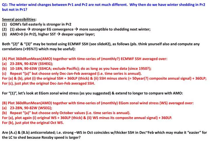
Q1: The winter wind changes between Pr1 and Pr2 are not much different. Why then do we have winter shedding in Pr2 but not in Pr1? • Several possibilities: • GOM’s fall easterly is stronger in Pr2 • (1) above stronger EG convergence more susceptible to shedding next winter; • AMO>0 (in Pr2), higher SST deeper upper layer; • Both “(2)” & “(3)” may be tested using ECMWF SSH (see slide#2), as follows (pls. think yourself also and compute any correlations (+95%!!) which may be useful): • (A) Plot 360dRunMean(AMO) together with time-series of (monthly?) ECMWF SSH averaged over: • 23-28N, 90-82W (SSHEG); • 10-18N, 90-63W (SSHCA; exclude Pacific); do as long as you have data (since 1950?); • Repeat “(a)” but choose only Dec-Jan-Feb averaged (i.e. time series is annual). • For (a) & (b), plot (i) the original SSH + 360LP (thick) & (ii) SSH minus steric (= 50year(?) composite annual signal) + 360LP; • For (c), just plot the original Dec-Jan-Feb averaged SSH. • For “(1)”, let’s look at EGom zonal wind stress (as you suggested) & extend to longer to compare with AMO: • (B) Plot 360dRunMean(AMO) together with time-series of (monthly) EGom zonal wind stress (WS) averaged over: • 23-28N, 90-82W (WSEG); • Repeat “(a)” but choose only October values (i.e. time series is annual). • For (a), plot again (i) original WS + 360LP (thick) & (ii) WS minus its composite annual signal) + 360LP. • For (b), just plot the original Oct WS. • Are (A.c) & (B.b) anticorrelated; i.e. strong –WS in Oct coincides w/thicker SSH in Dec~Feb which may make it “easier” for the LC to shed because Rossby speed is larger?
1988~2008 Monthly mean CCMP –Zonal wind NCEP Dp/Dy, dT/dy 1948~2010 Monthly mean NCEP –Zonal wind NCEP Dp/Dy, dT/dy