Download
1 / 22
341 likes | 668 Vues
Probabilistic Reasoning over Time. Russell and Norvig: ch 15. sensors. environment. ?. agent. actuators. Temporal Probabilistic Agent. t 1 , t 2 , t 3 , …. Time and Uncertainty. The world changes, we need to track and predict it Examples: diabetes management, traffic monitoring

E N D
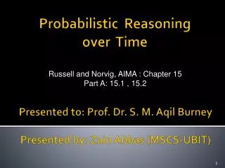
Probabilistic Reasoning over Time Russell and Norvig: ch 15
sensors environment ? agent actuators Temporal Probabilistic Agent t1, t2, t3, …
Time and Uncertainty • The world changes, we need to track and predict it • Examples: diabetes management, traffic monitoring • Basic idea: copy state and evidence variables for each time step • Xt – set of unobservable state variables at time t • e.g., BloodSugart, StomachContentst • Et – set of evidence variables at time t • e.g., MeasuredBloodSugart, PulseRatet, FoodEatent • Assumes discrete time steps
States and Observations • Process of change is viewed as series of snapshots, each describing the state of the world at a particular time • Each time slice involves a set or random variables indexed by t: • the set of unobservable state variables Xt • the set of observable evidence variable Et • The observation at time t is Et = et for some set of values et • The notation Xa:b denotes the set of variables from Xa to Xb
Stationary Process/Markov Assumption • Markov Assumption: Xt depends on some previous Xis • First-order Markov process: P(Xt|X0:t-1) = P(Xt|Xt-1) • kth order: depends on previous k time steps • Sensor Markov assumption:P(Et|X0:t, E0:t-1) = P(Et|Xt) • Assume stationary process: transition model P(Xt|Xt-1) and sensor model P(Et|Xt) are the same for all t • In a stationary process, the changes in the world state are governed by laws that do not themselves change over time
Which mode is right is determined by domain. Eg. If a particle is executing a random walk along the x-axis, changing its position by +/-1 at each time step, then using the x-coordinate as the state gives a first-order Markov process.
Complete Joint Distribution • Given: • Transition model: P(Xt|Xt-1) • Sensor model: P(Et|Xt) • Prior probability: P(X0) • Then we can specify complete joint distribution:
Example Raint-1 Raint Raint+1 Umbrellat-1 Umbrellat Umbrellat+1
Assumption modification • first-order Markov process is used in previous example • There are two possible fixes if the approximation proves too inaccurate: • 1. Increasing the order of the Markov process model. • Use second-order model by adding Raint-2as a parent of Rain, which might give slightly more accurate predictions (for example, in Palo ,Alto it very rarely rains more than two days in a row). • 2. Increasing the set of state variables. • For example, we could add Season{ to allow us to incorporate historical records of rainy seasons, or we could add Temperaturet, Humidityt and Pressuretto allow us to use a physical model of rainy conditions.
Note • adding state variables might improve the system's predictive power but also increases the prediction requirements • we now have to predict the new variables as well. • add new sensors (Eg. measurements of temperature and pressure
Example: robot wandering • Problem: tracking a robot wandering randomly on the X-Y plane • state variables: position and velocity • the new position can be calculated by Newton's laws • the velocity may change unpredictably • Eg. battery-powered robot’s velocity may be effected by a battery exhaustion
Example: robot wandering • Battery exhaustion depends on how much power was used by all previous maneuvers, the Markov property is violated. • Add charge level Batteryt as state variable • new model to predict Batterytfrom Batteryt-1and the velocity • New sensors for charge level
Inference Tasks • Filtering or monitoring: P(Xt|e1,…,et)computing current belief state, given all evidence to date • Prediction: P(Xt+k|e1,…,et) computing prob. of some future state • Smoothing: P(Xk|e1,…,et) computing prob. of past state (hindsight)(0≤k ≤t) • Most likely explanation: arg maxx1,..xtP(x1,…,xt|e1,…,et)given sequence of observation, find sequence of states that is most likely to have generated those observations.
Examples • Filtering: What is the probability that it is raining today, given all the umbrella observations up through today? • Prediction: What is the probability that it will rain the day after tomorrow, given all the umbrella observations up through today? • Smoothing: What is the probability that it rained yesterday, given all the umbrella observations through today? • Most likely explanation: if the umbrella appeared the first three days but not on the fourth, what is the most likely weather sequence to produce these umbrella sightings?
Filtering & Prediction • We use recursive estimation to compute P(Xt+1 | e1:t+1) as a function of et+1 and P(Xt | e1:t) • We can write this as follows: • P(et+l lXt+1) is obtainable directly from the sensor model • This leads to a recursive definition • f1:t+1 = FORWARD(f1:t:t,et+1)
Example: rain & umbrella p. 543 • Model,P(R0) =<0.5,0.5>
Smoothing • Compute P(Xk|e1:t) for 0<= k < t • Using a backward message bk+1:t = P(Ek+1:t | Xk), we obtain • P(Xk|e1:t) = f1:kbk+1:t • The backward message can be computed using • This leads to a recursive definition • Bk+1:t = BACKWARD(bk+2:t,ek+1:t) (15.7)
Example from R&N: p. 545 • computing the smoothed estimate for the probability of rain at t = 1, given the umbrella observations on days 1 and 2. According to E.15.7 Pluged into E.15.8
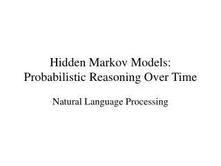
Probabilistic Temporal Models • Hidden Markov Models (HMMs) • Kalman Filters • Dynamic Bayesian Networks (DBNs)
Hidden Markov Models (HMMs) • Further simplification: • Only one state variable. • We can use matrices, now. • Ti,j = P(Xt=j|Xt-1=i) • Tijis the probability of a transition from state i to state j. • transition matrix for the umbrella world:
Hidden Markov Models (HMMs) • sensor model:diagonal matrix Ot • diagonal entries are given by the values P(et lXt = i) • Other entried:0 • Umbrella world
Hidden Markov Models (HMMs) Example: speech recognition