Download
1 / 53
550 likes | 692 Vues
Effect Size . More to life than statistical significance Reporting effect size. Statistical significance. Turns out a lot of researchers do not know what precisely p < .05 actually means Cohen (1994) Article: The earth is round (p<.05)

E N D
Effect Size More to life than statistical significance Reporting effect size
Statistical significance • Turns out a lot of researchers do not know what precisely p < .05 actually means • Cohen (1994) Article: The earth is round (p<.05) • What it means: "Given that H0 is true, what is the probability of these (or more extreme) data?” • Trouble is most people want to know "Given these data, what is the probability that H0 is true?"
Always a difference • With most analyses we commonly define the null hypothesis as ‘no relationship’ between our predictor and outcome(i.e. the ‘nil’ hypothesis) • With sample data, differences between groups always exist (at some level of precision), correlations are always non-zero. • Obtaining statistical significance can be seen as just a matter of sample size • Furthermore, the importance and magnitude of an effect are not accurately reflected because of the role of sample size in probability value attained
What should we be doing? • We want to make sure we have looked hard enough for the difference – power analysis • Figure out how big the thing we are looking for is – effect size
Calculating effect size • Though different statistical tests have different effect sizes developed for them, the general principle is the same • Effect size refers to the magnitude of the impact of some variable on another
Types of effect size • Two basic classes of effect size • Focused on standardized mean differences for group comparisons • Allows comparison across samples and variables with differing variance • Equivalent to z scores • Note sometimes no need to standardize (units of the scale have inherent meaning) • Variance-accounted-for • Amount explained versus the total • d family vs. r family • With group comparisons we will also talk about case-level effect sizes
Cohen’s d (Hedge’s g) • Cohen was one of the pioneers in advocating effect size over statistical significance • Defined d for the one-sample case
Cohen’s d • Note the similarity to a z-score- we’re talking about a standardized difference • The mean difference itself is a measure of effect size, however taking into account the variability, we obtain a standardized measure for comparison of studies across samples such that e.g. a d =.20 in this study means the same as that reported in another study
Cohen’s d • Now compare to the one-sample t-statistic • So • This shows how the test statistic (and its observed p-value) is in part determined by the effect size, but is confounded with sample size • This means small effects may be statistically significant in many studies (esp. social sciences)
Cohen’s d – Differences Between Means • Standard measure for independent samples t test • Cohen initially suggested could use either sample standard deviation, since they should both be equal according to our assumptions (homogeneity of variance) • In practice however researchers use the pooled variance
Example • Average number of times graduate psych students curse in the presence of others out of total frustration over the course of a day • Currently taking a statistics course vs. not • Data:
Example • Find the pooled variance and sd • Equal groups so just average the two variances such that and sp2 = 6.25
Cohen’s d – Differences Between Means • Relationship to t • Relationship to rpb P and q are the proportions of the total each group makes up. If equal groups p=.5, q=.5 and the denominator is d2 + 4 as you will see in some texts
Glass’s Δ • For studies with control groups, we’ll use the control group standard deviation in our formula • This does not assume equal variances
Dependent samples • One option would be to simply do nothing different than we would in the independent samples case, and treat the two sets of scores as independent • Problem: • Homogeneity of variance assumption may not be tenable • They aren’t independent
Dependent samples • Another option is to obtain a metric with regard to the actual difference scores on which the test is run • A d statistic for a dependent mean contrast is called a standardized mean change (gain) • There are two general standardizers: • A standard deviation in the metric of the • 1. difference scores (D) • 2. original scores
Dependent samples • Difference scores • Mean difference score divided by the standard deviation of the difference scores
Dependent samples • The standard deviation of the difference scores, unlike the previous solution, takes into account the correlated nature of the data • Var1 + Var2 – 2covar • Problems remain however • A standardized mean change in the metric of the difference scores can be much different than the metric of the original scores • Variability of difference scores might be markedly different for change scores compared to original units • Interpretation may not be straightforward
Dependent samples • Another option is to use standardizer in the metric of the original scores, which is directly comparable with a standardized mean difference from an independent-samples design • In pre-post types of situations where one would not expect homogeneity of variance, treat the pretest group of scores as you would the control for Glass’s Δ
Characterizing effect size • Cohen emphasized that the interpretation of effects requires the researcher to consider things narrowly in terms of the specific area of inquiry • Evaluation of effect sizes inherently requires a personal value judgment regarding the practical or clinical importance of the effects
How big? • Cohen (e.g. 1969, 1988) offers some rules of thumb • Fairly widespread convention now (unfortunately) • Looked at social science literature and suggested some ways to carve results into small, medium, and large effects • Cohen’s d values (Lipsey 1990 ranges in parentheses) • 0.2 small (<.32) • 0.5 medium (.33-.55) • 0.8 large (.56-1.2) • Be wary of “mindlessly invoking” these criteria • The worst thing that we could do is subsitute d = .20 for p = .05, as it would be a practice just as lazy and fraught with potential for abuse as the decades of poor practices we are currently trying to overcome
Small, medium, large? • Cohen (1969) • ‘small’ • real, but difficult to detect • difference between the heights of 15 year old and 16 year old girls in the US • Some gender differences on aspects of Weschler Adult Intelligence scale • ‘medium’ • ‘large enough to be visible to the naked eye’ • difference between the heights of 14 & 18 year old girls • ‘large’ • ‘grossly perceptible and therefore large’ • difference between the heights of 13 & 18 year old girls • IQ differences between PhDs and college freshman
Association • A measure of association describes the amount of the covariation between the independent and dependent variables • It is expressed in an unsquared standardized metric or its squared value—the former is usually a correlation*, the latter a variance-accounted-for effect size • A squared multiple correlation (R2) calculated in ANOVA is called the correlation ratio or estimated eta-squared (2)
Another measure of effect size • The point-biserial correlation, rpb, is the Pearson correlation between membership in one of two groups and a continuous outcome variable • As mentioned rpb has a direct relationship to t and d • When squared it is a special case of eta-squared in ANOVA • An one-way ANOVA for a two-group factor: eta-squared = R2 from a regression approach = r2pb
Eta-squared • A measure of the degree to which variability among observations can be attributed to conditions • Example: 2 = .50 • 50% of the variability seen in the scores is due to the independent variable.
Eta-squared • Relationship to t in the two group setting
Omega-squared • Another effect size measure that is less biased and interpreted in the same way as eta-squared
Partial eta-squared • A measure of the degree to which variability among observations can be attributed to conditions controlling for the subjects’ effect that’s unaccounted for by the model (individual differences/error) • Rules of thumb for small medium large: .01, .06, .14 • Note that in one-way design SPSS labels this as PES but is actually eta-squared, as there is only one factor and no others to partial out
Cohen’s f • Cohen has a d type of measuere for Anova called f • Cohen's f is interpreted as how many standard deviation units the means are from the grand mean, on average, or, if all the values were standardized, f is the standard deviation of those standardized means
Relation to PES Using Partial Eta-Squared
Guidelines • As eta-squared values are basically r2 values the feel for what is large, medium and small is similar and depends on many contextual factors • Small eta-squared and partial eta-square values might not get the point across (i.e. look big enough to worry about) • Might transform to Cohen’s f or use so as to continue to speak of standardized mean differences • His suggestions for f are: .10,.25,.40 which translate to .01,.06, and .14 for eta-squared values • That is something researchers could overcome if they understood more about effect sizes
Measures of association for non-continuous data Contingency coefficient Phi Cramer’s Phi d-family Odds Ratios Agreement Kappa Case level effect sizes Other effect size measures
Contingency Coefficient • An approximation of the correlation between the two variables (e.g. 0 to 1) • Problem- can’t ever reach 1 and its max value is dependent on the dimensions of the contingency table
Phi • Used in 2 X 2 tables as a correlation (0 to 1) • Problem- gets weird with more complex tables
Cramer’s Phi • Again think of it as a measure of association from 0 (weak) to 1 (strong), that is phi for 2X2 tables but also works for more complex ones. • k is the lesser of the number of rows or columns
Odds ratios • Especially good for 2X2 tables • Take a ratio of two outcomes • Although neither gets the majority, we could say which they were more likely to vote for respectively • Odds Clinton among Dems= 564/636 = .887 • Odds McCain among Reps= 450/550 = .818 • .887/.818 (the odds ratio) means they’d be 1.08 times as likely to vote Clinton among democrats than McCain among republicans • However, the 95% CI for the odds ratio is: • .92 to 1.28 • This suggests it would not be wise to predict either has a better chance at nomination at this point. • Numbers coming from • Feb 1-3 • Gallup Poll daily tracking. Three-day rolling average. N=approx. 1,200 Democrats and Democratic-leaning voters nationwide. • Gallup Poll daily tracking. Three-day rolling average. N=approx. 1,000 Republican and Republican-leaning voters nationwide.
Kappa Judgements by clinical psycholgists on the severity of suicide attempts by clients. At first glance one might think (10+5+3)/24 = 75% agreement between the two. However this does not take into account chance agreement. • Measure of agreement (from Cohen) • Though two folks (or groups of people) might agree, they might also have a predisposition to respond in a certain way anyway • Kappa takes this into consideration to determine how much agreement there would be after incorporating what we would expect by chance • O and E refer to the observed and expected frequencies on the diagonal of the table of Judge 1 vs Judge 2
Case-level effect sizes • Indexes such as Cohen’s d and eta2 estimate effect size at the group or variable level only • However, it is often of interest to estimate differences at the case level • Case-level indexes of group distinctiveness are proportions of scores from one group versus another that fall above or below a reference point • Reference points can be relative (e.g., a certain number of standard deviations above or below the mean in the combined frequency distribution) or more absolute (e.g., the cutting score on an admissions test)
Cohen’s (1988) measures of distribution overlap: U1 Proportion of nonoverlap If no overlap then = 1, 0 if all overlap U2 Proportion of scores in lower group exceeded by the same proportion in upper group If same means = .5, if all group2 exceeds group 1 then = 1.0 U3 Proportion of scores in lower group exceeded by typical score in upper group Same range as U2 Case-level effect sizes
Other case-level effect sizes • Tail ratios (Feingold, 1995): Relative proportion of scores from two different groups that fall in the upper extreme (i.e., either the left or right tail) of the combined frequency distribution • “Extreme” is usually defined relatively in terms of the number of standard deviations away from the grand mean • Tail ratio > 1.0 indicates one group has relatively more extreme scores • Here, tail ratio = p2/p1:
Other case-level effect sizes • Common language effect size (McGraw & Wong, 1992) is the predicted probability that a random score from the upper group exceeds a random score from the lower group • Find area to the right of that value • Range .5 – 1.0
Effect size statistics such as Hedge’s g and η2 have complex distributions Traditional methods of interval estimation rely on approximate standard errors assuming large sample sizes General form for d Confidence Intervals for Effect Size
Confidence Intervals for Effect Size • Standard errors
Problem • However, CIs formulated in this manner are only approximate, and are based on the central (t) distribution centered on zero • The true (exact) CI depends on a noncentral distribution and additional parameter • Noncentrality parameter • What the alternative hype distribution is centered on (further from zero, less belief in the null) • d is a function of this parameter, such that if ncp = 0 (i.e. is centered on the null hype value), then d = 0 (i.e. no effect)
Confidence Intervals for Effect Size • Similar situation for r and eta2 effect size measures • Gist: we’ll need a computer program to help us find the correct noncentrality parameters to use in calculating exact confidence intervals for effect sizes • Statistica has such functionality built into its menu system while others allow for such intervals to be programmed (even SPSS scripts are available (Smithson))
Limitations of effect size measures • Standardized mean differences: • Heterogeneity of within-conditions variances across studies can limit their usefulness—the unstandardized contrast may be better in this case • Measures of association: • Correlations can be affected by sample variances and whether the samples are independent or not, the design is balanced or not, or the factors are fixed or not • Also affected by artifacts such as missing observations, range restriction, categorization of continuous variables, and measurement error (see Hunter & Schmidt, 1994, for various corrections) • Variance-accounted-for indexes can make some effects look smaller than they really are in terms of their substantive significance
Limitations of effect size measures • How to fool yourself with effect size estimation: • 1. Examine effect size only at the group level • 2. Apply generic definitions of effect size magnitude without first looking to the literature in your area • 3. Believe that an effect size judged as “large” according to generic definitions must be an important result and that a “small” effect is unimportant (see Prentice & Miller, 1992) • 4. Ignore the question of how theoretical or practical significance should be gauged in your research area • 5. Estimate effect size only for statistically significant results
Limitations of effect size measures • 6. Believe that finding large effects somehow lessens the need for replication • 7. Forget that effect sizes are subject to sampling error • 8. Forget that effect sizes for fixed factors are specific to the particular levels selected for study • 9. Forget that standardized effect sizes encapsulate other quantities such as the unstandardized effect size, error variance, and experimental design • 10. As a journal editor or reviewer, substitute effect size magnitude for statistical significance as a criterion for whether a work is published • 11. Think that effect size = cause size