Download
1 / 59
600 likes | 742 Vues
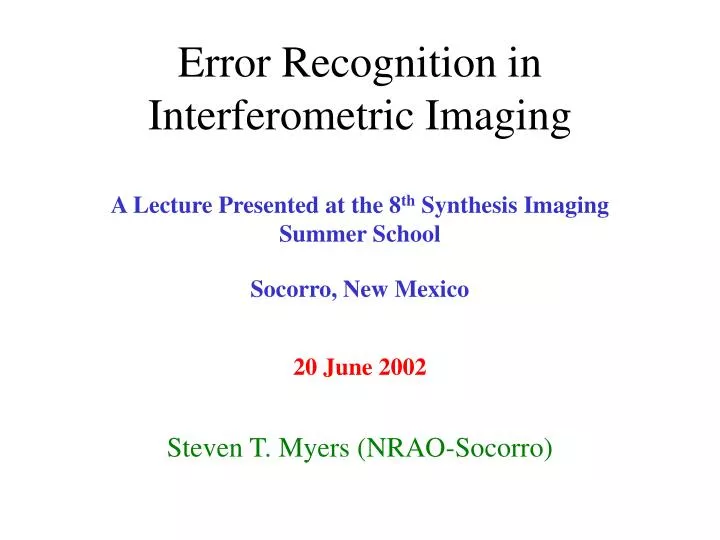
Error Recognition in Interferometric Imaging. A Lecture Presented at the 8 th Synthesis Imaging Summer School. Socorro, New Mexico. 20 June 2002. Steven T. Myers (NRAO-Socorro). Goals. Locate the causes of possible errors and defects Relate visibility errors to image defects

E N D
Error Recognition in Interferometric Imaging A Lecture Presented at the 8th Synthesis Imaging Summer School Socorro, New Mexico 20 June 2002 Steven T. Myers (NRAO-Socorro)
Goals Locate the causes of possible errors and defects Relate visibility errors to image defects Learn methods of diagnosing common problems Find solutions for correction of errors Figure out who to blame when you can’t fix it!
Where Are Errors Introduced? far field (atmosphere, ionosphere, beyond) near field (atmosphere, ionosphere) antenna frontend (optics, receiver) antenna backend (amplifiers, digitizers, etc.) baseline (correlator) post-correlation (computer, software, user)
Topography of the uv Plane • the sky has spherical geometry • spherical harmonics form complete basis • multipole expansion in l,m • at small angles this is Fourier transform in u,v • uv plane = “momentum space” • points in uv plane = plane waves on sky • effects in one domain mirror the other • “uncertainty principle”: localized broadened • truncation convolution
The Fourier Planes image plane and aperture (uv) planes are conjugate
Mosaicing synthesizing wider field narrows uv plane resolution
Image or Aperture Plane? • errors obey Fourier transform relations: • narrow features transform to wide features (and visa versa) • symmetries important (real/imag, odd/even, point/line/ring) • the transform of a serious error may not be serious! • effects are diluted by the number of other samples • watch out for short scans or effect on calibration solutions • some errors more obvious in particular domain • switch between image and uv planes
The 2D Fourier Transform x,y (radians) in tangent plane relative to phase center spatial frequency u,v (wavelengths) adopt the sign convention of Bracewell:
The Fourier Theorems shift in one domain is a phase gradient in the other multiplication in one domain is convolution in the other
Intensity and Visibility for a phase center at the pointing center xp primary beam pointing center phase center transform of primary beam frequency dependent true transform of sky brightness
Support in the uv Plane visibility = uv plane convolved with aperture x-cor
Fourier Symmetries • symmetries determined by Fourier kernel exp( if ) = cos f + i sin f • Real Real Even + Imag Odd • Imag Real Odd + Imag Even • Real & Even Real & Even • Real & Odd Imag & Odd • Even Even Odd Odd • real sky brightness Hermitian uv plane • complex conjugate of visibility used for inverse baseline image errors with odd symmetry or asymmetric often due to phase errors
Transform Pairs - 1 Figure used without permission from Bracewell (1986). For educational purposes only, do not distribute.
Transform Pairs - 2 Figure used without permission from Bracewell (1986). For educational purposes only, do not distribute.
Transform Pairs - 3 Figure used without permission from Bracewell (1986). For educational purposes only, do not distribute.
Transform Pairs - 4 Figure used without permission from Bracewell (1986). For educational purposes only, do not distribute.
Error Diagnosis • amplitude or phase errors: • phase errors usually asymmetric or odd symmetry • amplitude errors usually symmetric (even) • short duration errors: • localized in uv plane distributed in image plane • narrow extended orthogonal direction in image • long timescale errors: • ridge in uv plane corrugations in image • ring in uv plane concentric “Bessel” rings in image
Additive or Multiplicative? • some errors add to visibilities • additive in conjugate plane • examples: noise, confusion, interference, cross-talk • others multiply or convolve visibilities • multiplication convolution in conjugate planes • examples: sampling, primary beam, gain errors, atmosphere
Antenna Based Errors • often easier to diagnose in uv plane • typically due to single antenna: • short duration = pattern of baselines (six-pointed for VLA) • long duration = rings (concentric corrugations in image) • effect in image plane diluted by other antennas • factor Nbad / Ntot of baselines affected • many antenna-based errors obey closure relations and are self-calibratable
Closure Relations complex antenna voltage gain errors cancel out in special combinations of baselines:
Additive Errors • adds tovisibilities transform adds to image • unconnected to real sources in the image • may make “fake” sources • sources of additive errors: • interference (sources outside beam, RFI, cross-talk) • baseline-dependent errors • noise • short strong gain errors can appear to be additive
Noise in Images • computable from radiometer equation • you should know expected noise level given the conditions • unexpectedly high noise levels may indicate problems • additive, same uv distribution as data • will show same sidelobe pattern as real sources! • issues: • deconvolution will modify noise characteristics – beware! • self-calibration on weak sources can manufacture a fake source from noise (especially with short solution intervals)
Multiplicative Errors 1 • multiplies visibilities convolved with image • will appear to be “attached” to sources in the image • antenna gain calibration errors • sidelobe pattern (e.g. Y for short durations, ripples or rings for longer durations) • troposphere and ionosphere • troposphere: 8+ GHz, water vapor content plus dry atmosphere • ionosphere: < 8 GHz, total electron content (TEC) • antenna-based errors (usually closing), calibratable
Multiplicative Errors 2 • atmosphere and ionosphere (continued) • worse on longer baselines • short-term (sub-integration) errors smear image • long-term large-scale structures cause image shifts/distortions • phase gradient position shift (Fourier shift theorem) • equivalent to optical “seeing” • need phase referencing to calibrator(s) for astrometry • but, keep track of turns of phase! • wide-field: higher-order distortions over field of view • VLBI: incoherent between antennas – phase referencing needed
Multiplicative Errors 3 • uvsampling • sampling multiplicative with true uv distribution • sampling function dirty beam convolved with image • considered under Imaging & Deconvolution • primary beam and field-of-view • multiplicative in image plane convolves uv distribution • for baseline = cross-correlation of aperture voltage patterns • compact in uv plane extended sidelobes in image plane • can be corrected for in image plane by division (PBCOR) • can be compensated for in uv plane by mosaicing
uv Coverage snapshot coverage 8 scans over 10 hours
Radially Dependent Errors • not expressible as simple operations in image/uv plane • sometimes convertible to standard form via coordinate change • smearing effects • bandwidth: radial - like coadding images scaled by frequency • time-average: tangential – baselines rotated in uv plane • pointing • dependent on source position in the field • polarization effects worse (e.g. beam squint)
Example Error - 1 • point source 2005+403 • process normally • self-cal, etc. • introduce errors • clean no errors: max 3.24 Jy rms 0.11 mJy 6-fold symmetric pattern due to VLA “Y” 13 scans over 12 hours 10% amp error all ant 1 time rms 2.0 mJy
Example Error - 2 10 deg phase error 1 ant 1 time rms 0.49 mJy 20% amp error 1 ant 1 time rms 0.56 mJy anti-symmetric ridges symmetric ridges
Example Error - 3 10 deg phase error 1 ant all times rms 2.0 mJy 20% amp error 1 ant all times rms 2.3 mJy rings – odd symmetry rings – even symmetry
Editing – Search & Destroy! • For calibrators: be ruthless! • single errors can propagate to bad solutions which will affect longer intervals • may want to flag target source data around flagged calibrator scans • For target sources: keep in mind image-plane effect • single bad integrations highly diluted in image • long-term offsets can be more serious
Editing – What? • plot amplitude & phase versus time: • plot baselines versus a given antenna, look for outliers etc. • discriminates antenna-based and baseline-based errors • TVFLG (AIPS), msplot (aips++), vplot (difmap) • check different IF and polarization products • may be best to delete all data to a given antenna • for polarization observations, flag cross-hands (e.g. RL,LR) also when editing parallel hands (e.g. RR,LL)
Example Edit – msplot (2) Fourier transform of nearly symmetric planetary disk bad
Example Edit – TVFLG (1) AN9 bad IF2 AN1 AN2… Jupiter structure! time quack these! baseline bad
Example Edit – TVFLG (2) AN10 pointing? Q-Band AN16 low
More on Editing • editing tricks • also plot versus uv distance (e.g. UVPLT, msplot) • plot differences versus running mean (amplitude & phase) • antenna temperatures: e.g. TYPLT (AIPS) • calibration solutions: SNPLT (AIPS), plotcal (aips++) • also check IF 1-2 and R-L for anomalous jumps • special cases • spectral line: continuum versus line channels • VLBI: channels, delay and rate solutions • autocorrelations
Example Edit – TVFLG (3) AN23 problems amplitude differences quack these!
Example Edit – TVFLG (4) phase differences bad scan low amp phase noisy!
Example Edit - SNPLT 180 deg R-L phase jump in AN13
Interference 1 • strong additive errors • most often seen on short baselines • bright sources in sidelobes • Sun (and Cyg-A at low frequencies) can be seen even though the source may be offset by many primary beams! • watch for aliasing near map edge • radio frequency interference (RFI) • variable, often short duration bursts, sometimes CW • predominantly on baselines with low fringe rate (e.g. N-S) and when pointed at low elevation
Interference 2 • radio frequency interference (RFI) continued • usually narrow band - avoidable or excisable in high spectral resolution modes when isolated to a few channels • system must have high degree of linearity to deal with strong signals without saturation • cross-talk between antennas • short baselines, especially when shadowing occurs • delete baslines where an antenna is shadowed
Example RFI The spectrum above left shows VLA 74 MHz spectral data in the presence of a broad RFI feature. After hanning smoothing the data with time, the broad feature is effectively removed, leaving only narrow easily excisable features in the plot at the right. Spectral plots provided by Rick Perley
Other Problems • wide-field imaging and mosaicing • particularly susceptible to pointing errors and smearing • high-dynamic range imaging • all these problems will be exacerbated! • even weak errors (especially non-closing) will affect data • the most difficult type of problem • other issues or hints: • detection experiments for weak source forgiving
Other Suggestions • polarization as a diagnostic • polarization images of unpolarized sources useful • V images sometimes useful (depends on cal scheme) • also, look at differences between IFs or channels • low-resolution images good first step • image full field-of-view and sidelobes • find confusing sources or signature of RFI • FT errors in image back to uv plane • identify source (antennas, baselines, or integrations)
Summary • effect in image depends on effect in uv plane or time stream • understand the properties of the Fourier transform • errors may be additive, multiplicative, radially dependent • move between image and uv plane • effective editing • know expected noise levels, gauge severity in image • edit calibration scans carefully • image the full beam to look for confusing sources or RFI • use visualization tools (getting better all the time) • know the effects of the imaging & calibration algorithms
Extra - Snapshot Sequence • imaging and self-calibrating VLA snapshot • A-config, 8.4 GHz, 30 sec, 0.2” resolution, 0.4mJy rms • processed in difmap • special problems for snapshots: • poor uv coverage = high sidelobes • weak source, must be careful in self-calibration • modelfitting instead of cleaning – see talk by Pearson • point source nature makes this easier!
Snapshot 1 uv coverage
Snapshot 2 amplitude vs. uv radius