Download
1 / 54
540 likes | 672 Vues
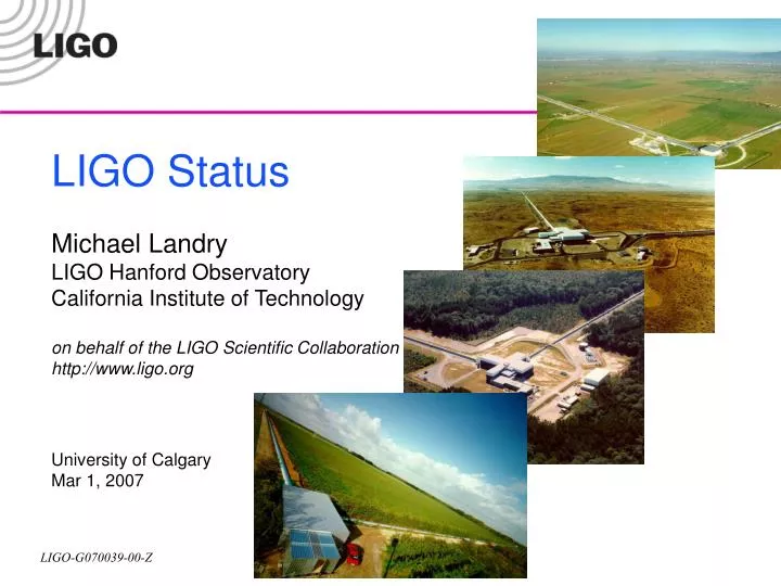
LIGO Status Michael Landry LIGO Hanford Observatory California Institute of Technology on behalf of the LIGO Scientific Collaboration http://www.ligo.org University of Calgary Mar 1, 2007. Challenges for a young field. First direct detection of gravitational waves

E N D
LIGO StatusMichael LandryLIGO Hanford ObservatoryCalifornia Institute of Technologyon behalf of the LIGO Scientific Collaborationhttp://www.ligo.orgUniversity of Calgary Mar 1, 2007
Challenges for a young field • First direct detection of gravitational waves • Detection possible with existing detectors • Probable with upgrades to existing facilities, and/or near-future new ones • Transition to a field of observational astronomy • EM emission – incoherent superposition of many emitters • Gravitational wave (GW) emission – coherently produced by bulk motions of matter • Matter is largely transparent to gravitational waves • Makes them hard to detect • Makes them a good probe of previously undetectable phenomena, e.g. dynamics of supernovae, black hole and neutron star mergers • Gravitational wave detectors are naturally all-sky devices; “pointing” can be done later in software
Overview • Introduction • What are gravitational waves, and what is the observable effect? • Sources • Hulse-Taylor binary pulsar • LIGO interferometers • Interferometric detectors. LIGO sites and installations. • Some topics in commissioning: the path to design sensitivity • Science mode running with LIGO, GEO and TAMA • Data analysis • Analyses from science runs for continuous wave sources, mostly. Inspiral, burst, stochastic if we have time. • Search for gravitational waves from known pulsars • Hierarchical search for unknown objects • Incoherent method • Coherent method
Overview • Introduction • What are gravitational waves, and what is the observable effect? • Sources • Hulse-Taylor binary pulsar • LIGO interferometers • Interferometric detectors. LIGO sites and installations. • Some topics in commissioning: the path to design sensitivity • Science mode running with LIGO, GEO and TAMA • Data analysis • Analyses from science runs for continuous wave sources, mostly. Inspiral, burst, stochastic if we have time. • Search for gravitational waves from known pulsars • Hierarchical search for unknown objects • Incoherent method • Coherent method
Gravitational waves • GWs are “ripples in spacetime”: rapidly moving masses generate fluctuations in spacetime curvature: • They are expected to propagate at the speed of light • They stretch and squeeze space
The two polarizations: the gravitational waveforms • The fields are described by 2 independent polarizations: h+(t)andhx(t) • The waveforms carry detailed information about astrophysical sources • With gravitational wave detectors one observes (a combination of) h+(t) and hx(t))
Example: Ring of test masses responding to wave propagating along z Amplitude parameterized by (tiny) dimensionless strain h: What is the observable effect?
Why look for gravitational radiation? • “Because it’s there!” • (George Mallory upon being asked, “why climb Everest?”) • Test General Relativity: • Quadrupolar radiation? Travels at speed of light? • Unique probe of strong-field gravity • Gain different view of Universe: • Sources cannot be obscured by dust / stellar envelopes • Detectable sources some of the most interesting, least understood in the Universe • Opens up entirely new non-electromagnetic spectrum. • May find something unexpected
What makes gravitational waves? • Compact binary inspiral: “chirps” • NS-NS waveforms are well described • BH-BH need better waveforms • Supernovae / GRBs: “bursts” • burst signals in coincidence with signals in electromagnetic radiation / neutrinos • all-sky untriggered searches too • Cosmological Signal: “stochastic background” • Pulsars in our galaxy:“continuous waves” • search for observed neutron stars • all-sky search (computing challenge)
Orbital decay:strong indirect evidence Emission of gravitational waves Neutron Binary System – Hulse & Taylor PSR 1913 + 16 -- Timing of pulsars 17 / sec · · ~ 8 hr • Neutron Binary System • separated by ~2x10⁶ km • m1 = 1.44m; m2 = 1.39m; e = 0.617 • Prediction from general relativity • spiral in by 3 mm/orbit • rate of change orbital period
Orbital decay:strong indirect evidence Emission of gravitational waves Neutron Binary System – Hulse & Taylor PSR 1913 + 16 -- Timing of pulsars 17 / sec See “Tests of General Relativity from Timing the Double Pulsar” Science Express, Sep 14 2006 The only double-pulsar system know, PSR J0737-3039A/B provides an update to this result. Orbital parameters of the double-pulsar system agree with those predicted by GR to 0.05% · · ~ 8 hr • Neutron Binary System • separated by ~2x10⁶ km • m1 = 1.44m; m2 = 1.39m; e = 0.617 • Prediction from general relativity • spiral in by 3 mm/orbit • rate of change orbital period
Overview • Introduction • What are gravitational waves, and what is the observable effect? • Sources • Hulse-Taylor binary pulsar • LIGO interferometers • Interferometric detectors. LIGO sites and installations. • Some topics in commissioning: the path to design sensitivity • Science mode running with LIGO, GEO and TAMA • Data analysis • Analyses from science runs for continuous wave sources, mostly. Inspiral, burst, stochastic if we have time. • Search for gravitational waves from known pulsars • Hierarchical search for unknown objects • Incoherent method • Coherent method
Gravitational wave detection • Suspended Interferometers • Suspended mirrors in “free-fall” • Michelson IFO is “natural” GW detector • Broad-band response (~50 Hz to few kHz) • Waveform information (e.g., chirp reconstruction) Fabry-Perot cavity 4km g.w. output port power recycling mirror • LIGO design length sensitivity: 10-18m
LIGO sites LIGO (Washington) (4km and 2km) LIGO (Louisiana) (4km) Funded by the National Science Foundation; operated by Caltech and MIT; the research focus for more than 500 LIGO Scientific Collaboration members worldwide.
The LIGO Observatories • Adapted from “The Blue Marble: Land Surface, Ocean Color and Sea Ice” at visibleearth.nasa.gov • NASA Goddard Space Flight Center Image by Reto Stöckli (land surface, shallow water, clouds). Enhancements by Robert Simmon (ocean color, compositing, 3D globes, animation). Data and technical support: MODIS Land Group; MODIS Science Data Support Team; MODIS Atmosphere Group; MODIS Ocean Group Additional data: USGS EROS Data Center (topography); USGS Terrestrial Remote Sensing Flagstaff Field Center (Antarctica); Defense Meteorological Satellite Program (city lights). LIGO Hanford Observatory (LHO) H1 : 4 km arms H2 : 2 km arms 10 ms LIGO Livingston Observatory (LLO) L1 : 4 km arms
Evacuated Beam Tubes Provide Clear Path for Light Vacuum required: <10-9 Torr
Evacuated Beam Tubes Provide Clear Path for Light • Bakeout facts: • 4 loops to return current, 1” gauge • 1700 amps to reach temperature • bake temp 140 degrees C for 30 days • 400 thermocouples to ensure even heating • each site has 4.8km of weld seams • full vent of vacuum: ~ 1GJ of energy Vacuum required: <10-9 Torr
Vacuum chambers provide quiet homes for mirrors The view inside the Corner Station Standing at the 4k vertex: beam splitter
damped springcross section Seismic Isolation – Springs and Masses
102 100 10-2 10-6 Horizontal 10-4 10-6 10-8 Vertical 10-10 LIGO detector facilities Seismic Isolation • Multi-stage (mass & springs) optical table support gives 106 suppression • Pendulum suspension gives additional 1 / f 2 suppression above ~1 Hz Transfer function Frequency (Hz)
All-Solid-State Nd:YAG Laser Custom-built 10 W Nd:YAG Laser, joint development with Lightwave Electronics (now commercial product) Cavity for defining beam geometry, joint development with Stanford Frequency reference cavity (inside oven)
Core optics suspension and control Optics suspended as simple pendulums Shadow sensors & voice-coil actuators provide damping and control forces Mirror is balanced on 30 micron diameter wire to 1/100th degree of arc
Interferometer length control system • Multiple Input / Multiple Output • Three tightly coupled cavities • Employs adaptive control system that evaluates plant evolution and reconfigures feedback paths and gains during lock acquisition 4km (photodiode)
Calibration of interferometer output • Combination of • Swept-Sine methods (accounts for gain vs. frequency) calibrate meters of mirror motion per count at digital suspension controllers across the frequency spectrum • DC measurements to set length scale (calibrates voice coil actuation of suspended mirror) • Calibration lines injected during running to monitor optical gain changes due to drift
Calibrated output: LIGO noise history Curves are calibrated interferometer output: spectral content of the gravity-wave channel
Noise component analysis from first science run (S1) LLO 4k Blue curve is calibrated interferometer output: spectral content of the gravity-wave channel S1 Measure and model noise contributions of various subsytems – understand your noise 5
Estimated noise limits for S2(as planned in October 2002) S1 S2 (expected from targeted improvements)
S1 S2 S3 S4 S5 - current 15Mpc Calibrated output: LIGO noise history 80kpc 1Mpc S1 S2 (improvements in sensitivity realized)
Now and then you get lucky • Near disaster: L1 ITMy got stuck- • Vented and fixed it: Noise got better!!! Earth quake stop before after
Tidal compensation data differential mode common mode Tidal evaluation on 21-hour locked section of S1 data Predicted tides Feedforward Feedback Residual signal on coils Residual signal on laser
LIGO/GEO/TAMA Science runs LIGO Hanford control room 31 Mar 2006 – S5
2 2 2 2 4 4 4 4 1 1 1 1 3 3 3 3 10-21 10-22 E3 E7 E5 E9 E10 E8 Runs S1 S2 S3 S4 S5 Science First Science Data Time line 2007 1999 2000 2001 2002 2003 2004 2005 2006 2 4 2 4 4 1 3 1 3 2 4 3 1 3 Inauguration First Lock Full Lock all IFO Now 4K strain noise at 150 Hz [Hz-1/2] 10-17 10-18 10-20 E2 E11 Engineering Coincident science runs with GEO and TAMA
LIGO, GEO S5 duty cycle S5 overall duty cycles: H1: 74% H2: 79% L1: 59% Percentage of 1-year LHO-LLO coincidence: 70% GEO: since May06 full attendance of S5: 91% duty cycle (143 days of total science time)
Overview • Introduction • What are gravitational waves, and what is the observable effect? • Sources • Hulse-Taylor binary pulsar • LIGO interferometers • Interferometric detectors. LIGO sites and installations. • Some topics in commissioning: the path to design sensitivity • Science mode running with LIGO, GEO and TAMA • Data analysis • Analyses from science runs for continuous wave sources, mostly. Inspiral, burst, stochastic if we have time. • Search for gravitational waves from known pulsars • Hierarchical search for unknown objects • Incoherent method • Coherent method
Analysis goal for S5: hierarchical search Search for continuous waves A B • Searches for g.w. : • Known pulsars • S4 all-sky (incoherent) • S3 all-sky (coherent) Mountain on neutron star Precessing neutron star Credits: A. image by Jolien Creighton; LIGO Lab Document G030163-03-Z. B. image by M. Kramer; Press Release PR0003, University of Manchester - Jodrell Bank Observatory, 2 August 2000. C. image by Dana Berry/NASA; NASA News Release posted July 2, 2003 on Spaceflight Now. D. image from a simulation by Chad Hanna and Benjamin Owen; B. J. Owen's research page, Penn State University. C Accreting neutron star D Oscillating neutron star LIGO-G060177-00-W
Analyses for continuous gravitational waves I • S5 Time domain analysis • Targeted search of known objects: 97 pulsars with rotational frequencies > 25 Hz at known locations with phase inferred from radio data (knowledge of some parameters simplifies analysis) from the Jodrell Bank Pulsar Group (JBPG) and/or ATNF catalogue • Limit this search to gravitational waves from a neutron star (with asymmetry about its rotational axis) emitted at twice its rotational frequency, 2*frot • Signal would be frequency modulated by relative motion of detector and source, plus amplitude modulated by the motion of the antenna pattern of the detector • Analyzed from 4 Nov 2005 - 17 Sep 2006 using data from the three LIGO observatories Hanford 4k and 2k (H1, H2) and Livingston 4k (L1) • Upper limits defined in terms of Bayesian posterior probability distributions for the pulsar parameters • Validation by hardware injection of fake pulsars • Results S5 data: first 10 months
CW source model • F+ and Fx : strain antenna patterns of the detector to plus and cross polarization, bounded between -1 and 1 • Here, signal parameters are: • h0 – amplitude of the gravitational wave signal • y – polarization angle of signal • i – inclination angle of source with respect to line of sight • f0 – initial phase of pulsar; F(t=0), and F(t)= f(t) + f0 The expected signal has the form: Heterodyne, i.e. multiply by: so that the expected demodulated signal is then: Here, a = a(h0, y, i, f0), a vector of the signal parameters.
Aside: Injection of fake pulsars during S2 Parameters of P1: Two simulated pulsars, P1 and P2, were injected in the LIGO interferometers for a period of ~ 12 hours during S2 P1: Constant Intrinsic Frequency Sky position: 0.3766960246 latitude (radians) 5.1471621319 longitude (radians) Signal parameters are defined at SSB GPS time 733967667.026112310 which corresponds to a wavefront passing: LHO at GPS time 733967713.000000000 LLO at GPS time 733967713.007730720 In the SSB the signal is defined by f = 1279.123456789012 Hz fdot = 0 phi = 0 psi = 0 iota = p/2 h0 = 2.0 x 10⁻²¹ phase j0 recovered amplitude h0 injected amplitude h0 y cos i
S5 Results, 95% upper limits PRELIMINARY • Lowest h0 upper limit: • PSR J1802-2124 (fgw = 158.1 Hz, r = 3.3kpc) h0 = 4.9x10⁻²⁶ • Lowest ellipticity upper limit: • PSR J2124-3358 (fgw = 405.6Hz, r = 0.25kpc)e = 1.1x10⁻⁷ All values assume I = 1038 kgm2 and no error on distance Our most stringent ellipticities (~10-7) are starting to reach into the range of neutron star structures for some neutron-proton-electron models (B. Owen, PRL, 2005).
Preliminary S5 result: known pulsars and 10 months of data PRELIMINARY
Frequency Time Time Analyses for continuous gravitational waves II • “Stack Slide Method”: break up data into segments; FFT each, producing Short (30 min) Fourier Transforms (SFTs) = coherent step. • StackSlide: stack SFTs, track frequency, slide to line up & add the power weighted by noise inverse = incoherent step. • Other semi-coherent methods: • Hough Transform: Phys. Rev. D72 (2005) 102004; gr-qc/0508065. • PowerFlux • Fully coherent methods: • Frequency domain match filtering/maximum likelihood estimation Track Doppler shift and df/dt
PRELIMINARY Analysis of Hardware Injections Fake gravitational-wave signals corresponding to rotating neutron stars with varying degrees of asymmetry were injected for parts of the S4 run by actuating on one end mirror. Sky maps for the search for an injected signal with h0 ~ 7.5e-24 are below. Black stars show the fake signal’s sky position. DEC (degrees) DEC (degrees) RA (hours) RA (hours) LIGO-G060177-00-W
S4 StackSlide “Loudest Events” 50-225 Hz PRELIMINARY • Searched 450 freq. per .25 Hz band, 51 values of df/dt, between 0 & -1e-8 Hz/s, up to 82,120 sky positions (up to 2e9 templates). The expected loudest StackSlide Power was ~ 1.22 (SNR ~ 7) • Veto bands affected by harmonics of 60 Hz. • Simple cut: if SNR > 7 in only one IFO veto; if in both IFOs, veto if abs(fH1-fL1) > 1.1e-4*f0 StackSlide Power StackSlide Power Frequency (Hz) LIGO-Gxxxxxx-00-W
S4 StackSlide “Loudest Events” 50-225 Hz PRELIMINARY • Searched 450 freq. per .25 Hz band, 51 values of df/dt, between 0 & -1e-8 Hz/s, up to 82,120 sky positions (up to 2e9 templates). The expected loudest StackSlide Power was ~ 1.22 (SNR ~ 7) • Veto bands affected by harmonics of 60 Hz. • Simple cut: if SNR > 7 in only one IFO veto; if in both IFOs, veto if abs(fH1-fL1) > 1.1e-4*f0 FakePulsar3=> FakePulsar8=> StackSlide Power <=Follow-up Indicates Instrument Line FakePulsar8=> StackSlide Power FakePulsar3=> <=Follow-up Indicates Instrument Line Frequency (Hz) LIGO-Gxxxxxx-00-W
S4 StackSlide h0 95% Confidence All Sky Upper Limits 50-225 Hz PRELIMINARY Best: 4.4e-24 For 139.5-139.75 Hz Band S5: ~ 2x better sensitivity, 12x or more data This incoherent method (and other examples, Hough and Powerflux techniques) is one piece of hierarchical pipeline h0 Upper Limit Best: 5.4e-24 For 140.75-141.0 Hz Band h0 Upper Limit LIGO-Gxxxxxx-00-W Frequency (Hz)
Analyses for continuous gravitational waves III • All-sky search is computationally intensive, e.g. • searching 1 year of data, you have 3 billion frequencies in a 1000Hz band • For each frequency we need to search 100 million million independent sky positions • pulsars spin down, so you have to consider approximately one billion times more templates • Number of templates for each frequency: ~1023 • S3 Frequency-domain (“F-statistic”) all-sky search • The F-Statistic uses a matched filter technique, minimizing chisquare (maximizing likelihood) when comparing a template to the data • ~1015 templates search over frequency (50Hz-1500Hz) and sky position • For S3 we are using the 600 most sensitive hours of data • We are combining the results of multiple stages of the search incoherently using a coincidence scheme
What would a pulsar look like? • Post-processing step: find points on the sky and in frequency that exceeded threshold in many of the sixty ten-hour segments • Software-injected fake pulsar signal is recovered below Simulated (software) pulsar signal in S3 data