Download
1 / 26
270 likes | 686 Vues
Sources of Market Risk. Decomposition. Losses can occur because of a combination of two factors: The exposure to the factor (a choice variable) The movement in the factor itself (which is external to the portfolio) Example: Fixed-coupon bond

E N D
Decomposition Losses can occur because of a combination of two factors: • The exposure to the factor (a choice variable) • The movement in the factor itself (which is external to the portfolio) Example: Fixed-coupon bond The potential for loss can be decomposed into the effect of dollar duration D*P and the changes in the yield dy dy / dp = -(D*P) dy = -(D*P)× dy(11.1) • It is possible to decompose the return on stock i into a market component and some residual risk Ri = αi + βi × RM + i ≈ βi × RM (11.2) αi is a constant: does not contribute to risk i specific risk that can be diversified Bahattin Buyuksahin, Celso Brunetti
Decomposition • Riis the rate of return no dimension To get a change in a dollar price, we write dPi =RiPiβi × Pi × RM (11.3) • Similarly, the change in the value of a derivative f can be expressed in terms of the change in the price of the underlying asset S, df / dS = df = × dS(11.4) • Notation: is the first partial derivative of the option • dfand dS are changes expressed in infinitesimal amounts • The change in value is linked to an exposure coefficient and a change in market variable: Market loss = Exposure × Adverse movement in financial variable Bahattin Buyuksahin, Celso Brunetti
Risk • First Moment: price movements St = $100, St+1 = $96 Returns: Rt = ln(St+1 / St) • Second Moment: Volatility Remember: usually we look at the volatility of the return process (not price) • Cross Movements: Correlations Remember: usually we look at the correlation of returns (not prices) Bahattin Buyuksahin, Celso Brunetti
Currency Risk: Price Movements Currency risk arises in the following environments • Pure currency float: the external value of a currency is free to move, to depreciate or appreciate market forces: example dollar/euro FX • Fixed currency system: a currency’s external value is fixed (or pegged) to another currency: example is the Hong Kong dollar, which is fixed against the U.S. dollar This does not mean there is no risk: possible readjustments in the parity value devaluations or revaluations • Change in currency regime: a currency that was previously fixed becomes flexible, or vice versa: example the Argentinian peso was fixed against the dollar until 2001 and floated thereafter Changes in regime can also lower currency risk, as in the recent case of the euro. Bahattin Buyuksahin, Celso Brunetti
Currency Risk: Volatility Bahattin Buyuksahin, Celso Brunetti
Currency Risk: Volatility Bahattin Buyuksahin, Celso Brunetti
Currency Risk: Correlation • Currency risk is also related to interest rate risk Often, interest rates are raised in an effort to stem the depreciation of a currency positive correlation between the currency and the bond market • Generally, correlations are low: -0.10 to 0.20 Diversification • Some correlations are high: currencies in the Euro area • Triangular Arbitrage: example S1 represents the dollar/pound rate and that S2 represents the dollar/euro (EUR) rate S3(EUR/BP) = S1($/BP)/S2($/EUR) • In Logs: ln[S3] = ln[S1] – ln[S2] (11.6) • Volatility: Bahattin Buyuksahin, Celso Brunetti
Fixed Income Risk • Fixed-income risk arises from movements in the level and volatility of bond yields yield curve risk Bahattin Buyuksahin, Celso Brunetti
Fixed Income Risk • Yields move because economic fundamentals are moving: Inflationary expectations Bahattin Buyuksahin, Celso Brunetti
Fixed Income Risk • The real interest rate is often defined as the nominal rate minus the rate of inflation rr,t = rn,t - t (1 + rr,t) = (1 + rn,t)/(1 + t ) This is generally positive but in recent years has been negative the Federal Reserve has kept nominal rates very low to stimulate economic activity • Movements in the term structure of interest rates are complex it is difficult to account for all the maturities market observers focus on a long-term rate (yield on the 10-year note) and a short-term rate (yield on a three-month bill) These two rates usefully summarize movements in the term structure • The two rates move in tandem, although the short-term rate displays higher volatility Spread is defined as the difference between the long rate and the short rate Periods of recession usually witness an increase in the term spread slow economic activity decreases the demand for capital, which in turn decreases short-term rates and increases the term spread Bahattin Buyuksahin, Celso Brunetti
Fixed Income Risk: Volatility • Bond returns volatility • Yield volatility: (dy) Bahattin Buyuksahin, Celso Brunetti
Fixed Income Risk: Correlation Bahattin Buyuksahin, Celso Brunetti
Fixed Income Risk: Correlation • Yield correlations are very high common factors • Combining Two Variables into a Single Factor: One can summarize the correlation between two variables in a scatter plot A regression line can then be fitted that represents the "best" summary of the linear relationship between the variables • Principal components is a statistical technique that extracts linear combinations of the original variables that explain the highest proportion of diagonal components of the matrix (Stevens, 1986) First principal component explains 94% of the total variance: level risk factor Second principal component explains 4% of the total variance: slope risk factor Third factor is found that represents a curvature risk factor Previous research: movements in yields could be usefully summarized by two to three factors that typically explain over 95% of the total variance Bahattin Buyuksahin, Celso Brunetti
Fixed Income Risk • Yield is very much linked to inflation Low (high) Yield low (high) expected inflation • Most bonds are issued in nominal terms nominal interest rate risk • Recently many countries have issued inflation-protected bonds, which make payments that are fixed in real terms but indexed to the rate of inflation the source of risk is real interest rate risk • Credit Spread Risk:A position in a credit spread can be established by investing in credit-sensitive bonds, such as corporate and shorting Treasuries with the appropriate duration If spread widen very high risk credit spreads increase in a recession and decrease in an expansion Bahattin Buyuksahin, Celso Brunetti
Equity Risk • Stock specific risk • Market risk • Stock market volatility: very high Bahattin Buyuksahin, Celso Brunetti
Commodity Risk • Commodity risk:movements in the value of commodity contracts Precious metals: gold, platinum, silver (volatility similar to equity markets) Base metals: aluminum, copper, nickel, zinc (volatility similar to equity markets) Energy products: natural gas, heating oil, unleaded gasoline, crude oil (very high volatility) • Futures risk exp(-y) y convenience yield Backwardation: S > F, Contango: S < F Bahattin Buyuksahin, Celso Brunetti
Diagonal Model: Sharpe • Decompose the stock return into two components: market and stock specific Assume i uncorrelated between each other and with the market V[Rp] = 2pV[RM] Bahattin Buyuksahin, Celso Brunetti
Diagonal Model: Sharpe • This consists of N elements in the vector β, N elements on the diagonal of the matrix D, plus the variance of the market itself The diagonal model reduces the number of parameters from N ×(N +1)/2 to 2N +1 if N = 100 from 5,050 parameters to 201 parameters Bahattin Buyuksahin, Celso Brunetti
Fixed Income Portfolio Risk • Decompose the movements in portfolio yield into three components: yi = zj + sk + i zj is the Treasury factor; sk is credit rating factor, i is the bond specific factor Define: DVBP as the dollar value of a basis point for a risk factor Bahattin Buyuksahin, Celso Brunetti
Fixed Income Portfolio Risk Bahattin Buyuksahin, Celso Brunetti