Download
1 / 58
580 likes | 737 Vues
Zero-Knowledge Proof System. Slides by Ouzy Hadad , Yair Gazelle & Gil Ben-Artzi Adapted from Ely Porat course lecture notes. Background and Motivation.

E N D
Zero-Knowledge Proof System Slides by Ouzy Hadad, Yair Gazelle & Gil Ben-Artzi Adapted from Ely Porat course lecture notes.
Background and Motivation • The purpose of a traditional proof is to convince somebody, but typically the details of a proof give the verifier more info about the assertion. • A proof is a zero-knowledge if the verifier does not get from it anything that he can not compute by himself.
Background and Motivation (cont.) • Whatever can be efficiently obtained by interacting with a prover, could also be computed without interaction, just by assuming that the assertion is true and conducting some efficient computation.
Zero Knowledge (Definition) • Let (P,V) be an interactive proof system for some language L. We say that (P,V), actually P, is zero-knowledge if for every probabilistic polynomial-time verifier V*, there exists a probabilistic polynomial-time machine M* s.t. for every xL holds • Machine M* is called the simulator for the interaction of V* with P.
Perfect Zero Knowledge (Definition) Let (P,V) be an interactive proof system for some language L. We say that (P,V), actually P, is perfect zero-knowledge (PZK) if for every probabilistic polynomial time verifier V*, there exists a probabilistic polynomial-time machine M* s.t. for every xLthe distributions{<P,V*>(x)}xLand{M*(x)}xLare identical,i.e.,
Statistically close distributions (Definition) The distribution ensembles {Ax}xL and{Bx}xLare statistically close or have negligible variation distance if for every polynomial p(•) there exits integerN such that for every xL with holds:
Statistical zero-knowledge (Definition) Let (P,V) be an interactive proof system for some language L. We say that (P,V), actually P, is statistical zero knowledge (SZK) if for every probabilistic polynomial time verifier V* there exists a probabilistic polynomial-time machine M* s.t. the ensembles {<P,V*>(x)}xLand{M*(x)}xLarestatistically close.
Computationally indistinguishable (Definition) Two ensembles {Ax}xL and{Bx}xL are computationally indistinguishable if for every probabilistic polynomial time distinguisher D and for every polynomial p(•) there exists an integer N such that for every xL with |x| N holds
Computational zero-knowledge (Definition) Let (P,V) be an interactive proof system for some language L. (P,V), actually P, is computational zero knowledge (CZK) if for every probabilistic polynomial-time verifier V* there exists a probabilistic polynomial-time machine M* s.t. the ensembles {<P,V*>(x)}xL and {M*(x)}xLare computationally indistinguishable.
PZK by view • The pair <P,V> is PZK by view if for every p.p.t V*... (probability polynomial time machine) there exist p.p.t M* such that for every xL we have: {view(P,V*)(x)={M*(x)} where view(P,V*)(x) is the view of V* after running <P,V*> on the input x, and M*(x) is the output of M* on the input x.
IP is PZK iff PZK by view Lemma: An interactive proof system is perfect zero-knowledge iff it is perfect zero knowledge by view. Proof: Let M* satisfy: {view<P,V*>(x)}xL {M*(x)}xL for every xL. M* has on its work-tape the final view of V*. Hence, it is able to perform the last step of V* and output the result. And so the modified M*(x) is identical to <P,V*>(x).
Proof of lemma (cont.) LetM* satisfy: {<P,V*>(x)}xL {M*(x)}xL . For a particular V*, let us consider a verifier V** that behaves exactly like V*, but outputs its whole view (at the end). There is a machine M** s.t.
Graph-Isomorphism • A pair of two graphs, Where • Lets be an isomorphism between the input graphs, namely is 1-1 and onto mapping of the vertex set V1 to the vertex set V2 so that
ZK proof for Graph Isomorphism • Prover’s first step(P1): Select random permutation over V1, construct the set , and send to the verifier. • Verifier’s first step gets H from P. select and send it to P. P is supposed to answer with an isomorphism between and .
ZK proof for Graph Isomorphism(cont.) (P2): If =1, then send = to V. Otherwise send = -1 to V. (V2): If is an isomorphism between G and H then V output 1, otherwise it outputs 0.
Construction (diagram) Prover Verifier =Random Permotation H G1 R{1,2} H If=1, send = otherwise = -1 Accept iff H = (G)
3 2 4 G2 4 5 5 1 G1 2 1 3 An example: Common input: two graphs G1 and G2. Only P knows.
An example (cont.) = -1 V sends =2 to P. 3 2 G2 4 2 5 5 4 1 G1 1 5 3 H 2 1 3 4 P sends Hto V. V gets and accepts. Only P knows.
Theorem: Graph isomorphism is in Zero-Knowledge Theorem 1: The construction above is a perfect zero-knowledge interactive proof system (with respect to statistical closeness).
Proof of Theorem 1 Completeness: If G1 G2 , V always accepts. First, G’=(G1). If =1 then = , Hence: (G) = (G1) = (G1) = G’ . If =2 then = -1, Hence: (G) = -1(G2) = (G1) = G’ . And hence V alwaysaccepts whenG1 G2 .
Proof of Theorem 1 (cont.) Soundness: Let P* be any prover. If it sends to V a graph not isomorphic neither to G1 nor to G2, then there is no isomorphism between G and G’. If G’ G1 then P* can convince V with probability at most 1/2 (V selects {1,2} uniformly). Hence: when G1 and G2 are non-isomorphic: If we will run this several times we will get the desire probability.
Zero Knowledge(Construction of a simulator) • Let V* be any polynomial-time verifier, and let q(•) be a polynomial bounding the running time of V*. • M* selects a string 01100…………011 = r
Construction of a Simulator (cont.) • M* selects R{1,2}. • M* selects a random permutation over V. • M*constructs G’’= (G). 4 2 5 G2 5 1 1 G’’ 3 2 3 4
Construction of a Simulator (cont.) • M* runs V* with the latter’s strings set as follows: • Denote as V*‘s output. Input Tape Random Tape x r G’’ Message Tape • M*halts with output(x,r,G’’,).
Proof of Theorem 1 (cont.) Definition: Let (P,V) be an interactive proof system for L. (P,V) is perfect zero-knowledge by view if for every probabilistic polynomial-time verifier V* there exists a probabilistic polynomial time machine M* s.t. for every xL holds: {view<P,V*>(x)}xL {M*(x)}xL where view<P,V*>(x) is the final view of V* after running <P,V*> on input x. view = all the data a machine possesses
Proof of Theorem 1 (cont.) Lemma:Then for every string r, graph H and permutation , it holds that: Pr [view<P,V*>(x) = (x,r,H,)] = Pr [M*(x) = (x,r,H,) | M*(x) ] Proof: Let m* describe M* conditioned on its not being . Define the 2 random variables: 1.v(x,r) - the last 2 elements of view(P,V*)(x) conditioned on the second element equals r. 2. (x,r) - the same with m*(x).
Proof of lemma (cont.) Let V* (x,r,H) denote the message sent by V* for a fixedr and an incoming message H. We will show that v(x,r) and (x,r) are uniformly distributed over the set: While running the simulator we have H=(G), and only the pairs satisfying =v*(x,r,H) lead to an output. Hence:
Proof of lemma (cont.) Consider v(x,r): For each H (which is isomorphic to G1): Observing that and hence the lemma follows.
Proof of Theorem 1 (cont.) Corollary:view<P,V*>(x) and M*(x) are statistically close. Proof: A failure is output with probability If the simulator returns steps P1-P2 of the construction |x| times and at least once at step P2 =, then output (x,r,G’’,). If in all |x| trials , then output rubbish. Hence, we got a statistical difference of and so the corollary follows.
Zero-Knowledge for NP NP Problem: A language L belongs to NP if and only if there exist a two-input polynomial-time algorithm A and constant C such that: there exist a certificate y with We say that algorithm A verifies language L in polynomial time.
IP for NP • Lets L language belong to NP, and x L , P should prove V that he know the solution for x. (P1): P guess the solution y for the problem x. (V1) V verify in polynomial time that A(x,y)=1. • We will give ZK interactive proof system for NP complete problem (G3C), which implies that for every NP problem, we have ZK proof.
G3C • Common Input: A graph 1 1 2 2 • P can paint the graph in 3 colors. 3 4 3 4 • P must keep the coloring a secret. 5 5
5 4 3 2 1 G3C is in Zero-Knowledge Construction (ZK IP for G3C): • P chooses a random color permutation. 1 1 2 2 3 3 4 4 • He puts all the nodes inside envelopes. 5 5 • And sends them to the verifier.
1 2 3 4 5 1 2 3 4 5 G3C is in ZK (cont.) • Verifier receives a 3-colored graph, but colors are hidden. • He chooses an edge at random. • And asks the prover to open the 2 envelopes.
1 2 3 G3C is in ZK (cont.) • Prover opens the envelopes, revealing the colors. 1 2 • Verifier accepts if the colors are different. 3 4 5
Formally, • G = (V,E) is 3-colorable if there exists a mapping for every . • Let be a 3-coloring of G, and let be a permutation over {1,2,3} chosen randomly. • Define a random 3-coloring. • Put each (v) in a box with v marked on it. • Send all the boxes to the verifier.
Formally, (cont.) • Verifier selects an edge at random asking to inspect the colors. • Prover sends the keys to boxes u and v. • Verifier uses the keys to open the boxes. • If he finds 2 different colors from {1,2,3} - Accept. • Otherwise - Reject.
Keyu , keyv P V G3C (diagram) 1 2 n (1) (2) (n) P V P V
The construction is in ZK: • Completeness:If G is 3-colorable and both P and V follow the rules, V will accept. • Soundness:Suppose G is not 3-colorable and P* tries to cheat. Then at least one edge (u,v) will be colored badly: (u) = (v).V will pick a bad edge with probability which can be increased to by repeating the protocol sufficiently many times.
Zero Knowledge(Construction of a simulator) • Let V* be any polynomial-time verifier, and let q(•) be a polynomial bounding the running time of V*. • M* selects a string
Construction of a Simulator (cont.) • M* selects e’=(u’,v’) R E. • M* sends to V* boxes filled with garbage, except for the boxes of u’ and v’, colored as follows: c d C R {1,2,3} d R {1,2,3}\{c} u’ v’ • If V* picks (u’,v’), M* sends V* their keys and the simulation is completed. • Otherwise, the simulation fails.
Analysis of the Simulation For every GG3C, the distribution of m*(<G>) = M*(<G>) | (M*(<G>) ) is identical to <P,V*>(<G>). Since V* can’t tell e’ from other edges by looking at the boxes, he picks e’ with probability 1/|E|, which can be increased to a constant by repeating M* sufficiently many times. So if the boxes are perfectly sealed, G3CPZK.
ZK for Finding square modulo n • Input: x2 modulo n . • output: x modulo n. • The prover need to prove that he know the output.
ZK for Finding square modulo n (cont.) (P1): P find two large prime number p,q, where n=p·q. He also choose randomly r [n, n4]. P sendn, x2 mod n and r2 mod n to V. (V1): V has two possibilities (a) Ask r. check the value of r2 mod n. (b) Ask for x ·r. check the value of x2r2 mod n
Analysis of the Protocol - square modulo n Soundness: If P does not know x, then in probability of 50% V will catch him, if we will run this several times we will get the V will reject in probability larger then 2/3. Completeness: If P know x, V always accept.
Analysis of the Protocol - square modulo n (cont.) • This protocol is computational ZK. • The Protocol give the value x2 mod n but the verifier can't calculate xfrom it . • If the verifier ask option 1 from the prover, he get no additional info. • If the verifier ask option 2 from the prover, he get xr which is random.
CO-NP ZK • In order to prove the above it’s enough to show that CO-NP complete problem is in IP • We will show that CO-SAT belongs to IP. • Than we can show that CO-SAT belongs to ZK. • Reminder: CO-SAT means that there are no truth assignment for an equation. • We can treat it as a specific case of proving that for an equation there are exactly K truth assignments (In this case , K=0)
CO-SAT IP • Lemma 1. (x1,x2,x3,…,Xn) has exactly Kn truth assignments k0,k1 : Kn=k0+k1 2. (0,x2,x3,…Xn) = 0(x2,x3,…Xn) has exactly k0 truth assignments 3. (1,x2,x3,…Xn) = 1(x2,x3,…Xn) has exactly k1 truth assignments • Informal explanation • By setting a variable in the original equations we create a new equation with a special relation to the original one. • Each new equation must have a specific number of assignments which can be pre-calculate.
CO-SAT IP • We can now construct a solution based upon the previous lemma • Prover will send verifier k0,k1 for (n) • Verifier will check that for (n-1) , condition 1 of lemma is true ( Kn=k0+k1) • Verifier will create randomly a new equation (n+1), by assigning 1 or 0 to the first variable of n • If we assign 1 , the number of solutions should be K0 , otherwise k0 • Verifier will send to prover the new equation
CO-SAT IP • Now prover will send the new k0n,k1n for the new (n+1) • Verifier remember previous k1 and can check if k1=k0n+k1n , so the prover cannot cheat him • Each stage we reduced one variable from equation by assign a value to it • Now let’s prove completeness & soundness