Download

1 / 42
420 likes | 555 Vues
09/23/10. Image Morphing. Computational Photography Derek Hoiem, University of Illinois. Many slides from Alyosha Efros. Project 2. Class choice awards Jia -bin Huang Guenther Charwat. All 2D Linear Transformations. Linear transformations are combinations of … Scale, Rotation,

E N D
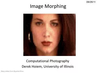
09/23/10 Image Morphing Computational Photography Derek Hoiem, University of Illinois Many slides from Alyosha Efros
Project 2 • Class choice awards • Jia-bin Huang • Guenther Charwat
All 2D Linear Transformations • Linear transformations are combinations of … • Scale, • Rotation, • Shear, and • Mirror • Properties of linear transformations: • Origin maps to origin • Lines map to lines • Parallel lines remain parallel • Ratios are preserved • Closed under composition
Affine Transformations Affine transformations are combinations of • Linear transformations, and • Translations Properties of affine transformations: • Origin does not necessarily map to origin • Lines map to lines • Parallel lines remain parallel • Ratios are preserved • Closed under composition Will the last coordinate w ever change?
Projective Transformations Projective transformations are combos of • Affine transformations, and • Projective warps Properties of projective transformations: • Origin does not necessarily map to origin • Lines map to lines • Parallel lines do not necessarily remain parallel • Ratios are not preserved • Closed under composition • Models change of basis • Projective matrix is defined up to a scale (8 DOF)
2D image transformations • These transformations are a nested set of groups • Closed under composition and inverse is a member
Recovering Transformations • What if we know f and g and want to recover the transform T? • e.g. better align images from Project 2 • willing to let user provide correspondences • How many do we need? ? T(x,y) y y’ x x’ f(x,y) g(x’,y’)
Translation: # correspondences? • How many correspondences needed for translation? • How many Degrees of Freedom? • What is the transformation matrix? ? T(x,y) y y’ x x’
Affine: # correspondences? • How many DOF for affine transform? • How many correspondences are needed? ? T(x,y) y y’ x x’
Take-home Question 9/23/2010 1) Suppose we have two triangles: ABC and A’B’C’. What transformation will map A to A’, B to B’, and C to C’? How can we get the parameters? B’ B ? T(x,y) C’ A C A’ Source Destination
Today: Morphing Women in art • http://youtube.com/watch?v=nUDIoN-_Hxs Aging http://www.youtube.com/watch?v=L0GKp-uvjO0
Image warping • Given a coordinate transform (x’,y’)=T(x,y) and a source image f(x,y), how do we compute a transformed image g(x’,y’)=f(T(x,y))? T(x,y) y y’ x x’ f(x,y) g(x’,y’)
Forward warping • Send each pixel f(x,y) to its corresponding location • (x’,y’)=T(x,y) in the second image T(x,y) y y’ x x’ f(x,y) g(x’,y’)
Forward warping • Send each pixel f(x,y) to its corresponding location • (x’,y’)=T(x,y) in the second image What is the problem with this approach? T(x,y) y y’ x x’ f(x,y) g(x’,y’) Q: what if pixel lands “between” two pixels? • A: distribute color among neighboring pixels (x’,y’) • Known as “splatting”
T-1(x,y) Inverse warping • Get each pixel g(x’,y’) from its corresponding location • (x,y)=T-1(x’,y’) in the first image y y’ x x x’ f(x,y) g(x’,y’) Q: what if pixel comes from “between” two pixels?
T-1(x,y) Inverse warping • Get each pixel g(x’,y’) from its corresponding location • (x,y)=T-1(x’,y’) in the first image y y’ x x x’ f(x,y) g(x’,y’) Q: what if pixel comes from “between” two pixels? • A: Interpolate color value from neighbors • nearest neighbor, bilinear, Gaussian, bicubic • Check out interp2 in Matlab
Bilinear Interpolation http://en.wikipedia.org/wiki/Bilinear_interpolation
Forward vs. inverse warping • Q: which is better? • A: Usually inverse—eliminates holes • however, it requires an invertible warp function
Morphing = Object Averaging • The aim is to find “an average” between two objects • Not an average of two images of objects… • …but an image of the average object! • How can we make a smooth transition in time? • Do a “weighted average” over time t
Averaging Points • P and Q can be anything: • points on a plane (2D) or in space (3D) • Colors in RGB or HSV (3D) • Whole images (m-by-n D)… etc. Q v= Q - P What’s the average of P and Q? P Extrapolation: t<0 or t>1 P+ 1.5v = P + 1.5(Q – P) = -0.5P+ 1.5 Q (t=1.5) P + 0.5v = P + 0.5(Q – P) = 0.5P + 0.5 Q Linear Interpolation New point: (1-t)P + tQ 0<t<1
Idea #1: Cross-Dissolve • Interpolate whole images: • Imagehalfway = (1-t)*Image1 + t*image2 • This is called cross-dissolve in film industry • But what if the images are not aligned?
Idea #2: Align, then cross-disolve • Align first, then cross-dissolve • Alignment using global warp – picture still valid
Dog Averaging • What to do? • Cross-dissolve doesn’t work • Global alignment doesn’t work • Cannot be done with a global transformation (e.g. affine) • Any ideas? • Feature matching! • Nose to nose, tail to tail, etc. • This is a local (non-parametric) warp
Idea #3: Local warp, then cross-dissolve • Morphing procedure • For every frame t, • Find the average shape (the “mean dog”) • local warping • Find the average color • Cross-dissolve the warped images
Local (non-parametric) Image Warping • Need to specify a more detailed warp function • Global warps were functions of a few (2,4,8) parameters • Non-parametric warps u(x,y) and v(x,y) can be defined independently for every single location x,y! • Once we know vector field u,v we can easily warp each pixel (use backward warping with interpolation)
Image Warping – non-parametric • Move control points to specify a spline warp • Spline produces a smooth vector field
Warp specification - dense • How can we specify the warp? Specify corresponding spline control points • interpolate to a complete warping function But we want to specify only a few points, not a grid
Warp specification - sparse • How can we specify the warp? Specify corresponding points • interpolate to a complete warping function • How do we do it? How do we go from feature points to pixels?
Triangular Mesh • Input correspondences at key feature points • Define a triangular mesh over the points • Same mesh (triangulation) in both images! • Now we have triangle-to-triangle correspondences • Warp each triangle separately from source to destination • How do we warp a triangle? • 3 points = affine warp!
Triangulations • A triangulation of set of points in the plane is a partitionof the convex hull to triangles whose vertices are the points, and do not contain other points. • There are an exponential number of triangulations of a point set.
An O(n3) Triangulation Algorithm • Repeat until impossible: • Select two sites. • If the edge connecting them does not intersect previous edges, keep it.
“Quality” Triangulations • Let (Ti) = (i1, i2,.., i3) be the vector of angles in the triangulation T in increasing order: • A triangulation T1is “better” than T2 if the smallest angle of T1 is larger than the smallest angle of T2 • Delaunay triangulation is the “best” (maximizes the smallest angles) good bad
Improving a Triangulation • In any convex quadrangle, an edge flip is possible. If this flip improves the triangulation locally, it also improves the global triangulation. If an edge flip improves the triangulation, the first edge is called “illegal”.
Illegal Edges • An edge pq is “illegal” iff one of its opposite vertices is inside the circle defined by the other three vertices (see Thale’s theorem) • A triangle is Delaunay iffno other points are inside the circle through the triangle’s vertices • The Delaunay triangulation is not unique if more than three nearby points are co-circular • The Delaunay triangulation does not exist if three nearby points are colinear p q
Naïve Delaunay Algorithm • Start with an arbitrary triangulation. Flip any illegal edge until no more exist. • Could take a long time to terminate.
Delaunay Triangulation by Duality • Draw the dual to the Voronoi diagram by connecting each two neighboring sites in the Voronoi diagram. • The DT may be constructed in O(nlogn) time • This is what Matlab’sdelaunay function uses
Image Morphing • We know how to warp one image into the other, but how do we create a morphing sequence? • Create an intermediate shape (by interpolation) • Warp both images towards it • Cross-dissolve the colors in the newly warped images
Warp interpolation How do we create an intermediate shape at time t? • Assume t = [0,1] • Simple linear interpolation of each feature pair • (1-t)*p1+t*p0 for corresponding features p0 and p1
Morphing & matting • Extract foreground first to avoid artifacts in the background Slide by Durand and Freeman
Dynamic Scene Black or White (MJ): http://www.youtube.com/watch?v=l6GJd8xoe0k Willow morph: http://www.youtube.com/watch?v=uLUyuWo3pG0
Summary of warping • Define corresponding points • Define triangulation on points • Use same triangulation for both images • For each t = 0:step:1 • Compute the average shape (weighted average of points) • For each triangle in the average shape • Get the affine projection to the corresponding triangles in each image • For each pixel in the triangle, find the corresponding points in each image and set value to weighted average (optionally use interpolation) • Save the image as the next frame of the sequence
Next class • “Fun with Faces” with Ali Farhadi • Project 3 due Monday