Download
1 / 57
590 likes | 773 Vues
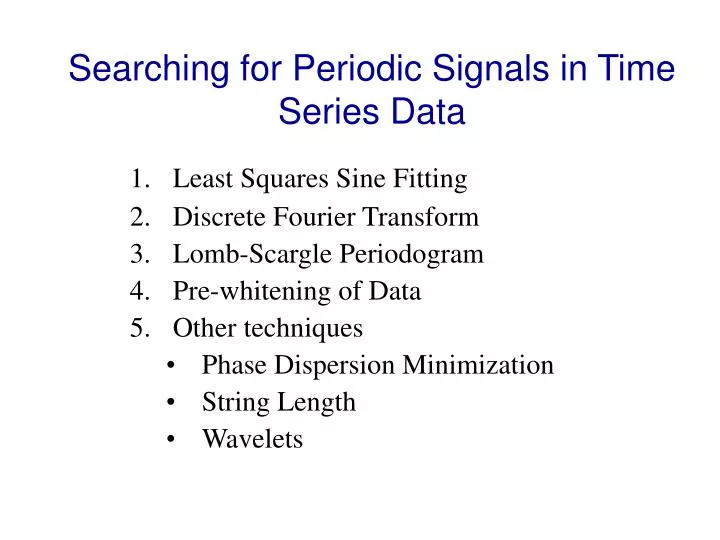
Searching for Periodic Signals in Time Series Data. Least Squares Sine Fitting Discrete Fourier Transform Lomb-Scargle Periodogram Pre-whitening of Data Other techniques Phase Dispersion Minimization String Length Wavelets. Period Analysis.

E N D
Searching for Periodic Signals in Time Series Data • Least Squares Sine Fitting • Discrete Fourier Transform • Lomb-Scargle Periodogram • Pre-whitening of Data • Other techniques • Phase Dispersion Minimization • String Length • Wavelets
Period Analysis How do you know if you have a periodic signal in your data? What is the period?
1. Least-squares Sine fitting • Fit a sine wave of the form: • V(t) = A·sin(wt + f) + Constant • Where w = 2p/P, f = phase shift • Best fit minimizes the c2: • c2 = S (di –gi)2/N • di = data, gi = fit
Advantages of Least Sqaures sine fitting: • Good for finding periods in relatively sparse data • Disadvantages of Least Sqaures sine fitting: • Signal may not always be a sine wave (e.g. eccentric orbits) • No assessement of false alarm probability (more later) • Don‘t always trust your results
This is fake data of pure random noise with a s = 30 m/s. Lesson: poorly sampled noise almost always can give you a period, but it it not signficant
1 N0 2. The Discrete Fourier Transform • Any function can be fit as a sum of sine and cosines N0 FT(w) = Xj (t) e–iwt Recall eiwt = cos wt + i sinwt j=1 X(t) is the time series Power: Px(w) = | FTX(w)|2 N0 = number of points 2 1 2 ( [( ] ) ) S S Px(w) = Xj cos wtj + Xj sin wtj N0 A DFT gives you as a function of frequency the amplitude (power) of each sine wave that is in the data
The continous form of the Fourier transform: F(s) = f(x) e–ixs dx f(x) = 1/2p F(s) eixs ds eixs = cos(xs) + i sin (xs) This is only done on paper, in the real world (computers) you always use a discrete Fourier transform (DFT)
The Fourier transform tells you the amplitude of sine (cosine) components to a data (time, pixel, x,y, etc) string Goal: Find what structure (peaks) are real, and what are artifacts of sampling, or due to the presence of noise
P Ao Ao t FT x 1/P w A pure sine wave is a delta function in Fourier space n 0 A constant value is a delta function with zero frequency in Fourier space: Always subtract off „dc“ level.
Useful concept: Convolution f(u)f(x–u)du = f * f f(x): f(x):
f(x-u) a2 a3 a1 a2 a3 a1 Useful concept: Convolution g(x) Convolution is a smoothing function
Convolution In Fourier space the convolution is just the product of the two transforms: Normal Space Fourier Space f*g F G
DFT of a pure sine wave: width Side lobes So why isn‘t it a d-function?
It would be if we measured the blue line out to infinity: But we measure the red points. Our sampling degrades the delta function and introduces sidelobes
× 0 * Dt 1/Dt × * = = 1/Dt 1/P In time space In Fourier Space 1/P
Window Data 16 min period sampled regularly for 3 hours
The longer the data window, the narrower is the width of the sinc function window:
Error in the period (frequency) of a peak in DFT: 3ps dn = 2 N1/2 T A s = error of measurement T = time span of your observations A = amplitude of your signal N = number of data points
A more realistic window And data
Alias periods: Undersampled periods appearing as another period
P –1 P –1 P –1 P –1 P –1 P –1 P –1 P –1 P –1 true alias true false false true false true false Alias periods: = + Common Alias Periods: + day (1 day)–1 = (29.53 d)–1 + month = year + (365.25 d)–1 =
Nyquist Frequency If T is your sampling rate which corresponds to a frequency of fs, then signals with frequencies up to fs/2 can be unambiguously reconstructed. This is the Nyquist frequency, N: N < fs/2 e.g. Suppose you observe a variable star once per night. Then the highest frequency you can determine in your data is 0.5 c/d = 2 days
Nyquist frequency n=0 n=0 n=0 -n0 -n0 +n0 +n0 positive n negative n positive n negative n When you do a DFT on a sine wave with a period = 10, sampling = 1: n0=0.1, 1/Dt = 1
The effects of noise: Real Peaks s =10 m/s s =50 m/s s =100 m/s s =200 m/s 2 sine waves ampltudes of 100 and 50 m/s. Noise added at different levels
1 1 2 2 2 [ ] S 2 Xj cos w(tj–t) [ ] S Xj sin w(tj–t) j S j Xj cos2w(tj–t) S Xj sin2w(tj–t) j 3. Lomb-Scargle Periodograms Px(w) = + (Scos 2wtj) tan(2wt) = (Ssin 2wtj)/ j j Power is a measure of the statistical significance of that frequency (period): Scargle, Astrophysical Journal, 263, 835, 1982
Power: DFT versus Scargle DFT Scargle N=15 Scargle Power Amplitude (m/s) N=40 N=100 Frequency (c/d) DFTs give you the amplitude of a periodic signal in the data. This does not change with more data. The Lomb-Scargle power gives you the statistical significance of a period. The more data you have the more significant the detection is, thus the higher power with more data
False Alarm Probability (FAP) The FAP is the probability that random noise will produce a peak with Lomb-Scargle Power the same as your observed peak in a certain frequency range Unknown period: Where P = Scargle Power N = number of independent frequencies in the frequency range of interest FAP ≈ 1 – (1–e–P)N Known period: In this case you have only one independent frequency FAP ≈ e–P Scargle Power (significance) is increased by lower level of noise and/or more data points
False Alarm Probability (FAP) The probability that noise can produce the highest peak over a range ≈ 1 – (1–e–P)N FAP ≈ e–P The probability that noise can produce the this peak exactly at this frequency = e–P
Why is the FAP Impotant? Example: A transit candidate from BEST Depth [%] 1.2 Duration [h] ? Orbital period [d] Semi mayor axis[AU] Number of detections 1 Target field No. 8 Host star K...(?) Magnitude(B.E.S.T.) 11.25 Radius[Rsun] 0.65-0.85 Radius of planet ? [RJup] 0.71-0.89? To confirm you need radial velocity measurements, but you do not have a period… DSS1/POSSI
16 one-hour observations made with the 2m coude echelle 16 one hour observations made with the
Published (Dreizler et al. 2003) Radial Velocity Curve of the transiting planet OGLE 3 Wrong Phase (by 180 degrees) for a transiting planet!
Discovery of a rapidly oscillating Ap star with 16.3 min period FAP ≈ 10–5
b CrB Small FAP does not always mean a real signal Period = 11.5 min FAP = 0.015 Period = 16.3 min FAP = 10–5 Lesson: Do not believe any FAP < 0.01 My limit: < 0.001 Better to miss a real period than to declare a false one
Determining FAP: To use the Scargle formula you need the number of independent frequencies. How do you get the number of independent Frequencies? First Approximation: Use the number of data points N0 Horne & Baliunas (1986, Astrophysical Journal, 302, 757): Ni = –6.362 + 1.193 N0 + 0.00098N02= number of independent frequencies
Use Scargle FAP only as an estimate. A more valid determination of the FAP requires Monte Carlo Simulations: Method 1: • Create random noise at the same level as your data • Sample the random noise in the same manner as your data • Calculate Scargle periodogram of noise and determine highest peak in frequency range of interest • Repeat 1.000-100.000 times = Ntotal • Add the number of noise periodograms with power greater than your data = Nnoise • FAP = Nnoise/Ntotal Assumes Gaussian noise. What if your noise is not Gaussian, or has some unknown characteristics?
Use Scargle FAP only as an estimate. A more valid determination of the FAP requires Monte Carlo Simulations: Method 2: • Randomly shuffle the measured values (velocity, light, etc) keeping the times of your observations fixed • Calculate Scargle periodogram of random data and determine highest peak in frequency range of interest • Reshuffle your data 1.000-100.000 times = Ntotal • Add the number of „random“ periodograms with power greater than your data = Nnoise • FAP = Nnoise/Ntotal Advantage: Uses the actual noise characteristics of your data
FAP comparisons Scargle formula using N as number of data points Monte Carlo Simulation Using formula and number of data points as your independent frequencies may overestimate FAP, but each case is different.
Amplitude = level of noise 1 2 4 8 10 Amplitude/error 6 N = 20 Number of measurements needed to detect a signal of a certain amplitude. The FAP of the detection is 0.001. The noise level is s = 5 m/s. Basically, the larger the measurement error the more measurements you need to detect a signal.
Lomb-Scargle Periodogram of 6 data points of a sine wave: Lots of alias periods and false alarm probability (chance that it is due to noise) is 40%! For small number of data points do not use Scargle, sine fitting is best. But be cautious!!
Least squares sine fitting: The best fit period (frequency) has the lowest c2 Discrete Fourier Transform: Gives the power of each frequency that is present in the data. Power is in (m/s)2 or (m/s) for amplitude Amplitude (m/s) Lomb-Scargle Periodogram: Gives the power of each frequency that is present in the data. Power is a measure of statistical signficance
4. Finding Multiple Periods in Data: Pre-whitening What if you have multiple periods in your data? How do you find these and make sure that these are not due to alias effects of your sampling window. Standard procedure: Pre-whitening. Sequentially remove periods from the data until you reach the level of the noise
Prewhitening flow diagram: Find highest peak in DFT/Scargle (Pi) Save Pi Fit sine wave to data and subtract fit Calculate new DFT Are more peaks above the level of the noise? no Stop, publish all Pi yes
False alarm probability ≈ 10–14 Alias Peaks Noise level
Raw data After removal of dominant period False alarm probability ≈ 0.24
Useful program for pre-whitening of time series data: http://www.univie.ac.at/tops/Period04/ • Program picks highest peak, but this may be an alias • Peaks may be due to noise. A FAP analysis will tell you this
Amplitude Phase 5. Other Techniques: Phase Dispersion Minimization Wrong Period Correct Period Choose a period and phase the data. Divide phased data into M bins and compute the standard deviation in each bin. If s2 is the variance of the time series data and s2 the total variance of the M bin samples, the correct period has a minimum value of Q : Q = s2/s2 See Stellingwerf, Astromomical Journal, 224, 953, 1978