DENSITY LIMITS IN HARD DRIVES?

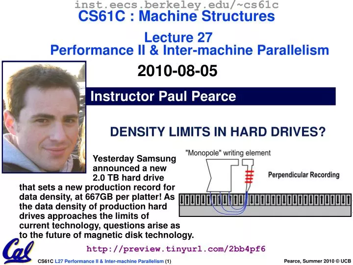
1. inst.eecs.berkeley.edu/~cs61cCS61C : Machine StructuresLecture 27 Performance II & Inter-machine Parallelism2010-08-05 Instructor Paul Pearce DENSITY LIMITS IN HARD DRIVES? Yesterday Samsung announced a new 2.0 TB hard drive that sets a new production record for data density, at 667GB per platter! As the data density of production hard drives approaches the limits of current technology, questions arise as to the future of magnetic disk technology. http://preview.tinyurl.com/2bb4pf6

2. “And in review…” • I/O gives computers their 5 senses • Vast I/O speed range • Processor speed means must synchronize with I/O devices before use • Polling works, but expensive • processor repeatedly queries devices • Interrupts works, more complex • devices causes an exception, causing OS to run and deal with the device • Latency v. Throughput • Real Time: time user waits for program to execute: depends heavily on how OS switches between tasks • CPU Time: time spent executing a single program: depends solely on design of processor (datapath, pipelining effectiveness, caches, etc.)

3. Performance Calculation (1/2) CPU execution time for program [s/p] =Clock Cycles for program [c/p] x Clock Cycle Time [s/c] Substituting for clock cycles: CPU execution time for program [s/p] =( Instruction Count[i/p] x CPI [c/i] ) x Clock Cycle Time [s/c] =Instruction Count x CPIx Clock Cycle Time

4. CPU time = Instructions Cycles Seconds Program Instruction Cycle CPU time = Instructions Cycles Seconds Program Instruction Cycle CPU time = Instructions Cycles Seconds Program Instruction Cycle CPU time = Seconds Program Performance Calculation (2/2)       Product of all 3 terms: if missing a term, can’tpredict time, the real measure of performance

5. How Calculate the 3 Components? • Clock Cycle Time: in specification of computer (Clock Rate in advertisements) • Instruction Count: • Count instructions in a small program by hand • Use simulator to count instructions • Hardware counter in spec. register (Pentium 4, Core 2 Duo, Core i7’s) to count both # of instructions and # of clock cycles. • CPI: • Calculate: Execution Time / Clock cycle time Instruction Count • Hardware counters also exist for number of CPU cycles, which can be used with the hardware counter for the number of instruction to calculate CPI. • Check the bonus slides for yet another way

6. What Programs Measure for Comparison? • Ideally run typical programs with typical input before purchase, or before even build machine • Called a “workload”; For example: • Engineer uses compiler, spreadsheet • Author uses word processor, drawing program, compression software • In some situations its hard to do • Don’t have access to machine to “benchmark” before purchase • Don’t know workload in future

7. Benchmarks • Obviously, apparent speed of processor depends on code used to test it • Need industry standards so that different processors can be fairly compared • Companies exist that create these benchmarks: “typical” code used to evaluate systems • Need to be changed every ~5 years since designers could (and do!) target for these standard benchmarks

8. Example Standardized Benchmarks (1/2) • Standard Performance Evaluation Corporation (SPEC) SPEC CPU2006 • CINT2006 12 integer (perl, bzip, gcc, go, ...) • CFP2006 17 floating-point (povray, bwaves, ...) • All relative to base machine (which gets 100)Sun Ultra Enterprise 2 w/296 MHz UltraSPARC II • They measure • System speed (SPECint2006) • System throughput (SPECint_rate2006) • www.spec.org/osg/cpu2006/

9. Example Standardized Benchmarks (2/2) • SPEC • Benchmarks distributed in source code • Members of consortium select workload • 30+ companies, 40+ universities, research labs • Compiler, machine designers target benchmarks, so try to change every 5 years • SPEC CPU2006: CFP2006bwaves Fortran Fluid Dynamics gamess Fortran Quantum Chemistry milc C Physics / Quantum Chromodynamics zeusmp Fortran Physics / CFD gromacs C,Fortran Biochemistry / Molecular Dynamics cactusADM C,Fortran Physics / General Relativity leslie3d Fortran Fluid Dynamics namd C++ Biology / Molecular Dynamics dealll C++ Finite Element Analysis soplex C++ Linear Programming, Optimization povray C++ Image Ray-tracing calculix C,Fortran Structural Mechanics GemsFDTD Fortran Computational Electromegnetics tonto Fortran Quantum Chemistry lbm C Fluid Dynamics wrf C,Fortran Weather sphinx3 C Speech recognition CINT2006perlbench C Perl Programming language bzip2 C Compression gcc C C Programming Language Compiler mcf C Combinatorial Optimization gobmk C Artificial Intelligence : Go hmmer C Search Gene Sequence sjeng C Artificial Intelligence : Chess libquantum C Simulates quantum computer h264ref C H.264 Video compression omnetpp C++ Discrete Event Simulation astar C++ Path-finding Algorithms xalancbmk C++ XML Processing

10. Administrivia • Project 3 due Monday August 9th @ midnight • Don’t forget to register your iClicker • http://www.iclicker.com/registration/ • Final is Thursday, August 12th 8am-11am • 1 Week from today! • Course Evaluations on Monday, please attend!

11. An overview of Inter-machine Parallelism • Amdahl’s Law • Motivation for Inter-machine Parallelism • Inter-machine parallelism hardware • Supercomputing • Distributed computing • Grid computing • Cluster computing • Inter-machine parallelism examples • Message Passing Interface (MPI) • Google’s MapReduce paradigm • Programming Challenges

12. Speedup Issues: Amdahl’s Law • Applications can almost never be completely parallelized; some serial code remains • s is serial fraction of program, P is # of processors • Amdahl’s law: Speedup(P) = Time(1) / Time(P) ≤ 1 / ( s+ [ (1-s) / P) ], and as P ∞ ≤ 1 / s • Even if the parallel portion of your application speeds up perfectly, your performance may be limited by the sequential portion Time Parallel portion Serial portion 1 2 3 4 5 Number of Processors

13. Big Problems • Simulation: the Third Pillar of Science • Traditionally perform experiments or build systems • Limitations to standard approach: • Too difficult – build large wind tunnels • Too expensive – build disposable jet • Too slow – wait for climate or galactic evolution • Too dangerous – weapons, drug design • Computational Science: • Simulate the phenomenon on computers • Based on physical laws and efficient numerical methods

14. Example Applications • Science & Medicine • Global climate modeling • Biology: genomics; protein folding; drug design; malaria simulations • Astrophysical modeling • Computational Chemistry, Material Sciences and Nanosciences • SETI@Home : Search for Extra-Terrestrial Intelligence • Engineering • Semiconductor design • Earthquake and structural modeling • Fluid dynamics (airplane design) • Combustion (engine design) • Crash simulation • Computational Game Theory (e.g., Chess Databases) • Business • Rendering computer graphic imagery (CGI), ala Pixar and ILM • Financial and economic modeling • Transaction processing, web services and search engines • Defense • Nuclear weapons -- test by simulations • Cryptography

15. Performance Requirements Performance terminology the FLOP: FLoating point OPeration “flops” = # FLOP/second is the standard metric for computing power Example: Global Climate Modeling Divide the world into a grid (e.g. 10 km spacing) Solve fluid dynamics equations for each point & minute Requires about 100 Flops per grid point per minute Weather Prediction (7 days in 24 hours): 56 Gflops Climate Prediction (50 years in 30 days): 4.8 Tflops Perspective Pentium 4 3GHz Desktop Processor ~10 Gflops Climate Prediction would take ~50-100 years www.epm.ornl.gov/chammp/chammp.html Reference:http://www.hpcwire.com/hpcwire/hpcwireWWW/04/0827/108259.html

16. High Resolution Climate Modeling on NERSC-3P. Duffy, et al., LLNL

17. What Can We Do? Use Many CPUs! • Supercomputing – like those listed in top500.org • Multiple processors “all in one box / room” from one vendor that often communicate through shared memory • This is often where you find exotic architectures • Distributed computing • Many separate computers (each with independent CPU, RAM, HD, NIC) that communicate through a network • Grids (heterogenous computers across Internet) • Clusters (mostly homogeneous computers all in one room) • Google uses commodity computers to exploit “knee in curve” price/performance sweet spot • It’s about being able to solve “big” problems, not “small” problems faster • These problems can be data (mostly) or CPU intensive

18. Distributed Computing Themes • Let’s network many disparate machines into one compute cluster • These could all be the same (easier) or very different machines (harder) • Common themes • “Dispatcher” gives jobs & collects results • “Workers” (get, process, return) until done • Examples • SETI@Home, BOINC, Render farms • Google clusters running MapReduce

19. Distributed Computing Challenges • Communication is fundamental difficulty • Distributing data, updating shared resource, communicating results • Machines have separate memories, so no usual inter-process communication – need network • Introduces inefficiencies: overhead, waiting, etc. • Need to parallelize algorithms • Must look at problems from parallel standpoint • Tightly coupled problems require frequent communication (more of the slow part!) • We want to decouple the problem • Increase data locality • Balance the workload

20. Programming Models: What is MPI? • Message Passing Interface (MPI) • World’s most popular distributed API • MPI is “de facto standard” in scientific computing • C and FORTRAN, ver. 2 in 1997 • What is MPI good for? • Abstracts away common network communications • Allows lots of control without bookkeeping • Freedom and flexibility come with complexity • 300 subroutines, but serious programs with fewer than 10 • Basics: • One executable run on every node • Each node process has a rank ID number assigned • Call API functions to send messages http://www.mpi-forum.org/ http://forum.stanford.edu/events/2007/plenary/slides/Olukotun.ppt http://www.tbray.org/ongoing/When/200x/2006/05/24/On-Grids

21. Challenges with MPI • Deadlock is possible… • Seen in CS61A – state of no progress • Blocking communication can cause deadlock • Large overhead from comm. mismanagement • Time spent blocking is wasted cycles • Can overlap computation with non-blocking comm. • Load imbalance is possible! Dead machines? • Things are starting to look hard to code!

22. A New Choice: Google’s MapReduce • Remember CS61A? (reduce + (map square '(1 2 3)) (reduce + '(1 4 9)) 14 • We told you “the beauty of pure functional programming is that it’s easily parallelizable” • Do you see how you could parallelize this? • What if the reduce function argument were associative, would that help? • Imagine 10,000 machines ready to help you compute anything you could cast as a MapReduce problem! • This is the abstraction Google is famous for authoring(but their reduce not the same as the CS61A’s or MPI’s reduce) • Often, their reducebuilds a reverse-lookup table for easy query • It hides LOTS of difficulty of writing parallel code! • The system takes care of load balancing, dead machines, etc.

23. MapReduce Programming Model Input & Output: each a set of key/value pairs Programmer specifies two functions: map (in_key, in_value)  list(out_key, intermediate_value) • Processes input key/value pair • Produces set of intermediate pairs reduce (out_key, list(intermediate_value))  list(out_value) • Combines all intermediate values for a particular key • Produces a set of merged output values (usually just one) code.google.com/edu/parallel/mapreduce-tutorial.html

24. MapReduce WordCount Example • “Mapper” nodes are responsible for the map function • // “I do I learn”  (“I”,1), (“do”,1), (“I”,1), (“learn”,1) map(String input_key, String input_value): // input_key : document name (or line of text) // input_value: document contentsfor each word w in input_value: EmitIntermediate(w, "1"); • “Reducer” nodes are responsible for the reducefunction • // (“I”,[1,1])  (“I”,2) reduce(String output_key, Iterator intermediate_values): // output_key : a word // output_values: a list of countsint result = 0; for each v in intermediate_values: result += ParseInt(v); Emit(AsString(result)); • Data on a distributed file system (DFS)

25. MapReduce Example Diagram file1 file2 file3 file4 file5 file6 file7 ah ah er ah ifor oruh or ah if map(String input_key, String input_value): // input_key : doc name // input_value: doc contentsfor each word w in input_value: EmitIntermediate(w, "1"); ah:1 if:1or:1 or:1uh:1 or:1 ah:1 if:1 ah:1 ah:1 er:1 ah:1,1,1,1 er:1 if:1,1 or:1,1,1 uh:1 reduce(String output_key, Iterator intermediate_values): // output_key : a word // output_values: a list of countsint result = 0; for each v in intermediate_values: result += ParseInt(v); Emit(AsString(result)); 4 1 2 3 1 (ah) (er) (if) (or) (uh)

26. MapReduce Advantages/Disadvantages • Now it’s easier to program some problems with the use of distributed computing • Communication management effectively hidden • I/O scheduling done for us • Fault tolerance, monitoring • machine failures, suddenly-slow machines, etc are handled • Can be much easier to design and program! • Can cascade several (many?) MapReduce tasks • But … it further restricts solvable problems • Might be hard to express problem in MapReduce • Data parallelism is key • Need to be able to break up a problem by data chunks • MapReduce is closed-source (to Google) C++ • Hadoop is open-source Java-based rewrite

27. So… What does it all mean? • Inter-machine parallelism is hard! • MPI and MapReduce are programming models that help us solve some distributed systems problems. • In general, there is no one “right” solution to inter-machine parallelism. • Next time, we’ll talk about Intra-machine parallelism (hint: also hard, see ParLab), or parallelism within one machine.

28. Peer Instruction A program runs in 100 sec. on a machine, mult accounts for 80 sec. of that. If we want to make the program run 6 times faster, we need to up the speed of mult by AT LEAST 6. The majority of the world’s computing power lives in supercomputer centers 12 a) FF b) FT c) TF d) TT

29. CPU time = Instructions x Cycles x Seconds Program Instruction Cycle “And in conclusion…” • Performance doesn’t depend on any single factor: need Instruction Count, Clocks Per Instruction (CPI) and Clock Rate to get valid estimations • Benchmarks • Attempt to predict perf, Updated every few years • Measure everything from simulation of desktop graphics programs to battery life • Megahertz Myth • MHz ≠ performance, it’s just one factor • And….

30. Also in conclusion… • Parallelism is necessary • It looks like it’s the future of computing… • It is unlikely that serial computing will ever catch up with parallel computing • Software parallelism • Grids and clusters, networked computers • Two common ways to program: • Message Passing Interface (lower level) • MapReduce (higher level, more constrained) • Parallelism is often difficult • Speedup is limited by serial portion of code and communication overhead

31. Bonus slides • These are extra slides that used to be included in lecture notes, but have been moved to this, the “bonus” area to serve as a supplement. • The slides will appear in the order they would have in the normal presentation Bonus

32. Calculating CPI Another Way • First calculate CPI for each individual instruction (add, sub, and, etc.) • Next calculate frequency of each individual instruction • Finally multiply these two for each instruction and add them up to get final CPI (the weighted sum)

33. (Where time spent) Instruction Mix Calculating CPI Another Way Example (RISC processor) Op Freqi CPIi Prod (% Time) ALU 50% 1 .5 (23%) Load 20% 5 1.0 (45%) Store 10% 3 .3 (14%) Branch 20% 2 .4 (18%) 2.2 • What if Branch instructions twice as fast?

34. Performance Evaluation: The Demo If we’re talking about performance, let’s discuss the ways shady salespeople have fooled consumers (so you don’t get taken!) 5. Never let the user touch it 4. Only run the demo through a script 3. Run it on a stock machine in which “no expense was spared” 2. Preprocess all available data 1. Play a movie

35. To Learn More… • About MPI… • www.mpi-forum.org • Parallel Programming in C with MPI and OpenMP by Michael J. Quinn • About MapReduce… • code.google.com/edu/parallel/mapreduce-tutorial.html • labs.google.com/papers/mapreduce.html • lucene.apache.org/hadoop/index.html

36. Basic MPI Functions (1) • MPI_Send() and MPI_Receive() • Basic API calls to send and receive data point-to-point based on rank (the runtime node ID #) • We don’t have to worry about networking details • A few are available: blocking and non-blocking • MPI_Broadcast() • One-to-many communication of data • Everyone calls: one sends, others block to receive • MPI_Barrier() • Blocks when called, waits for everyone to call (arrive at some determined point in the code) • Synchronization

37. Basic MPI Functions (2) • MPI_Scatter() • Partitions an array that exists on a single node • Distributes partitions to other nodes in rank order • MPI_Gather() • Collects array pieces back to single node (in order)

38. Basic MPI Functions (3) • MPI_Reduce() • Perform a “reduction operation” across nodes to yield a value on a single node • Similar to accumulate in Scheme • (accumulate + ‘(1 2 3 4 5)) • MPI can be clever about the reduction • Pre-defined reduction operations, or make your own (and abstract datatypes) • MPI_Op_create() • MPI_AllToAll() • Update shared data resource

39. MPI Program Template • Communicators - set up node groups • Startup/Shutdown Functions • Set up rank and size, pass argc and argv • “Real” code segment main(int argc, char *argv[]){MPI_Init(&argc, &argv); MPI_Comm_rank(MPI_COMM_WORLD, &rank); MPI_Comm_size(MPI_COMM_WORLD, &size);/* Data distribution */ ... /* Computation & Communication*/ ... /* Result gathering */ ...MPI_Finalize();}

40. MapReduce WordCount Java code

41. MapReduce in CS61A (and CS3?!) • Think that’s too much code? • So did we, and we wanted to teach the Map/Reduce programming paradigm in CS61A • “We” = Dan, Brian Harvey and ace undergrads Matt Johnson, Ramesh Sridharan, Robert Liao, Alex Rasmussen. • Google & Intel gave us the cluster you used in Lab! • You live in Scheme, and send the task to the cluster in the basement by invoking the fn mapreduce. Ans comes back as a stream. • (mapreduce mapper reducer reducer-base input) • www.eecs.berkeley.edu/Pubs/TechRpts/2008/EECS-2008-34.html

42. Our Scheme MapReduce interface