Download
1 / 45
450 likes | 456 Vues
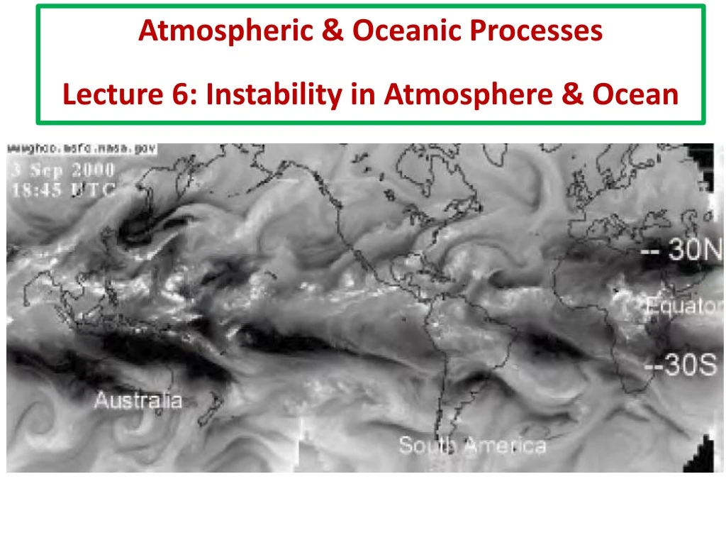
Atmospheric & Oceanic Processes Lecture 6: Instability in Atmosphere & Ocean. Fluid Convection. Schematic of shallow convection in a fluid , such as water, triggered by warming from below and/or cooling from above.

E N D
Atmospheric & Oceanic ProcessesLecture 6: Instability in Atmosphere & Ocean
Fluid Convection Schematic of shallow convection in a fluid, such as water, triggered by warming from below and/or cooling from above. When a fluid such as water is heated from below (or cooled from above), it develops overturning motions. This seems obvious. A thought experiment: consider the shallow, horizontally infinite fluid shown in Figure above. Let the heating be applied uniformly at the base; then the fluid should have a horizontally uniform temperature, so T = T(z) only. The fluid will be top-heavy: warmer and therefore lighter fluid below cold, dense fluid above. The situation does not contradict hydrostacy: ∂p/∂z = -gρ. BUT, 1. Why do motions develop when we can have hydrostatic equilibrium, with no net forces? 2. Why can the motions become horizontally inhomogeneous when the heating is horizontally uniform? Answer: because the “top-heavy” state of the fluid is unstable
Understanding instability x δx Stability and instability of a ball on a curved surface. Consider point “A” or “B”. Is the state of the ball stable? When perturbed, if the ball moves farther and farther from its original position, then unstable; otherwise stable. δθδh/δx Accx/(-g) So, Accx = d2x/dt2is: d2x/dt2 -g dh/dx δθ δh Accx -g δθ For small distances x from “A” (or “B”), acceleration is d2x/dt2;thereforealong the slope: d2x/dt2=−gdh/dx
Consider point “A” or “B” – is the state of the ball stable? When perturbed, if the ball moves farther and farther from its original position, then unstbale; otherwise the system is stable. For small distances x from “A” (or “B”), acceleration is d2x/dt2;thereforealong the slope: d2x/dt2=−gdh/dx = −g(d2h/dx2)Ax (Taylor expansion about “A” where dh/dx = 0) Solution is: x ~ exp(.t) where = [−g(d2h/dx2)A]1/2 Thus: at “A” where (d2h/dx2) < 0, the solution has an exponentially growing part, indicating instability; at “B” the solution is oscillatory, but stable. When the ball is perturbed from the crest (top of hill) it moves downslope, its potential energy decreases and its kinetic energy increases– unstable. In the valley, by contrast, one must keep on supplying potential energy to push the ball up, for otherwise it will sink back to the valley – stable.
Buoyancy in water – an incompressible fluid A parcel of light, buoyant fluid surrounded by resting, homogeneous, heavier fluid in hydrostatic balance, ∂p/∂z = -gρ. The fluid above points A1, A, and A2 has the same density, and hence, by hydrostacy, pressures at the A points are all the same. But the pressure at B is lower than at B1 or B2 because the column of fluid above B is lighter. There is thus a pressure gradient force which drives fluid inwards toward B (blue arrows), tending to equalize the pressure along B1BB2. The pressure just belowB will tend to increase, forcing the light fluid upward, as indicated schematically by the red arrows. The (upward) acceleration or buoyancy (b; note it is positive) of the parcel of fluid is: b = -gρ/ρP, ρ= ρP - ρE i.e. parcel minus environment densities.
Stability of a parcel in water Consider a fluid parcel initially at z1in an environment whose density is ρ(z) (see Figure on right). The parcel’s density ρ1 = ρ(z1), is the same as its environment at height z1. The parcel is now displaced without loosing or gaining heat (i.e. adiabatically), and also without expanding or contracting (incompressible), a small vertical distance to z2 = z1+ δz, where the new environment density is: ρE= ρ(z2) ρ1 + (dρ/dz)Eδz. The parcel’s buoyancy is then: b = -g(ρ1- ρE)/ρ1 = g(dρ/dz)Eδz /ρ1. Therefore, if (dρ/dz)E> 0 parcel keeps rising unstable (dρ/dz)E= 0 parcel stays neutrally stable (dρ/dz)E< 0 parcel returns stable An incompressible liquid is unstable if density increases with height (in the absence of viscous and diffusive effects)
Homework: stability using potential energy (PE) argument Homework #6.1 Consider again the Figure on right. Imagine that the 2 fluid parcels (“1” and “2”) exchange their positions. Before the exchange, the PE (focusing on these 2 parcels) is: PEbefore = g (ρ1z1 + ρ2z2) After the exchange: PEafter= g (ρ1z2+ ρ2z1). Show that the change in PE after the exchange is: PE = −g (ρ2 − ρ1) (z2 − z1) Then show: PE = -g(dρ/dz)E(z2– z1)2 . Then deduce and explain the stabilityand instability of the system based on the sign of PE. (Potential Energy)/Volume = ρgz
Laboratory experiment of convection Parcels overshoot Gravity waves 32 oC 14 oC c) (a) A sketch of the laboratory apparatus used to study convection. A stable stratification is set up in a 50cm × 50 cm × 50 cm tank by slowly filling it up with water whose temperature is slowly increased with time. This is done using (1) a mixer, which mixes hot and cold water together, and (2) a diffuser, which floats on the top of the rising water and ensures that the warming water floats on the top without generating turbulence. Using the hot and cold water supply we can achieve a temperature difference of 20◦C over the depth of the tank. The temperature profile is measured and recorded using thermometers attached to the side of the tank. Heating at the base is supplied by a heating pad. The motion of the fluid is made visible by sprinkling a very small amount of potassium permanganate (which turns the water pink) after the stable stratification has been set up and just before turning on the heating pad. Convection carries heat from the heating pad into the body of the fluid, distributing it over the convection layer much like convection carries heat away from the Earth’s surface. (b) Schematic of evolving convective boundary layer heated from below. The initial linear temperature profile is TE. The convection layer is mixed by convection to a uniform temperature. Fluid parcels overshoot into the stable stratification above, creating the inversion evident in (c). Both the temperature of the convection layer and its depth slowly increase with time.
Laboratory experiment: more discussions Heating starts 5 4 3 2 1 Parcels overshoot Gravity waves 5 Heating 4 3 Left: Parcels overshoot the neutrally buoyant level, brush the stratified layer above, produce gravity waves, then sink back into the convective layer beneath Right: Temperature time series measured by five thermometers spanning the depth of the fluid at equal intervals shown on left. The lowest thermometer is close to the heating pad. We see that the ambient fluid initially has a roughly constant stratification, somewhat higher near the top than in the body of the fluid. The heating pad was switched on at t = 150 sec. Note how all the readings converge onto one line as the well mixed convection layer deepens over time. 2 1
Appendix: Law of vertical heat transport Heat flux up = 0.5*ρrefcp(T+ T)wc H = heat flux = amount of heat transported across unit volume in unit time = (ρcpT)w (For water: cp= 4000 J kg−1 K−1) Cooler: T Heat flux down = 0.5*ρrefcpwcT Warmer: T+ T So, net heat flux, averaged horizontally, is H = (flux up – flux down) = 0.5*ρrefcpwcT. (Note T > 0). As light fluid rises and dense fluid sinks, PE = −g (ρ2 − ρ1) (z2 − z1) = -gρz KE = 3 × 0.5*ρrefwc2 (assuming isotropic motion – same in all 3 directions) So, wc2 (2/3).αgzT(α = -(/T)/o) i.e. H= 0.5*ρrefcpwcT 0.5*ρrefcp[(2/3).αgz]1/2T3/2 . In the laboratory experiment, the heating coil provides H = 4000 W m−2. If the convection penetrates over a vertical scale z = 0.2 m, then using α = 2 × 10⁻⁴ K−1 and cp= 4000 J kg−1 K−1, we obtain: T 0.1K and wc 0.5 cm s−1.
Stability of a dry & compressibleatmosphere The real atmosphere is compressible, so that e.g. an air parcel can expand when experiencing less pressure, i.e. its density not only depends on T, but also on pressure p. As the parcel rises, it moves into an environment of lower pressure. The parcel will adjust to this pressure; in doing so it will expand, doing work on its surroundings, and thus cool. For dry parcel, its temperature drops like: dT/dz= − g/cp= −Γd, Γdis the dry adiabatic lapse rate= the rate at which the parcel’s temperature decreases with height under adiabatic displacement. Derive above using 1st law of thermodynamics, equation of state for ideal dry air and hydrostatic equation. As the air parcel rises, expands and cools, we can compare its temperature with that of the environment (E) whose temperature drops with height like (dT/dz)E. If after the parcel cools, it is still warmer than the new surrounding at the greater height, then the parcel will keep on rising, and the atmosphere is unstable. This will occur if: (dT/dz)E < -Γd Unstable. Otherwise: (dT/dz)E > -Γd Stable. Homework #6.2
dp/dz= -ρg p = ρRT If incompressible, then ρ = constant, and dp/dz = ρRdT/dz = -ρg so that dT/dz = -g/R But if air is compressible, then: dT/dz = -g/(R+Cv) = -g/Cp --- *** (see Lecture#2 for the relation between Cv , Cp and R). For derivation of ***, see my notes on next slide Solution to Homework #6.2
Stability of a dry & compressibleatmosphere (cont’d) Thus for convection to occur, it is not enough for the atmosphere’s temperature to decrease with height, it must decrease faster than the rate at which an air parcel’s temperature decreases with height as the parcel expands – this rate is called the Dry Adiabatic Lapse Rate = -g/cp10 K km−1, using cp= 1005 J kg−1K−1 for air. The atmosphere is nearly always stable to dry processes. A parcel displaced upwards (downwards) in an adiabatic process moves along a dry adiabat (the dotted line) and cools down (warms up) at a rate that is faster than that of the environment, ∂TE/∂z. Since the parcel always has the same pressure as the environment, it is not only colder (warmer) but also denser (lighter). The parcel therefore experiences a force pulling it back toward its reference height.
Stability of a dry & compressibleatmosphere (cont’d) Thus for convection to occur, it is not enough for the atmosphere’s temperature to decrease with height, it must decrease faster than the rate at which an air parcel’s temperature decreases with height as the parcel expands – this rate is called the Dry Adiabatic Lapse Rate = -g/cp10 K km−1, using cp= 1005 J kg−1K−1 for air. In the tropic, the atmosphere (dT/dz)E -4.6 K km−1, so it is actually stable to dry convection. Homework #6.3 Using the “T” profile shown on left figure, and the hydrostatic equation, show that (dT/dz)E -4.6 K km−1. 270 K 295 K
The zonally-averaged Potential Temperature for annual (top), DJF (middle) and JAS (bottom).
Stability of a dry & compressibleatmosphere (concluded) Thus for convection to occur, it is not enough for the atmosphere’s temperature to decrease with height, it must decrease faster than the rate at which an air parcel’s temperature decreases with height as the parcel expands – this rate is called the Dry Adiabatic Lapse Rate = -g/cp10 K km−1, using cp= 1005 J kg−1K−1 for air. In the tropic, the atmosphere has (dT/dz)E-4.6 K km−1, so it is actually stable to dry convection. It is the release of latent heat which makes the air parcel unstable: Moist Adiabatic Lapse Rate 3K km−1.
10 km 5 km 200 K 250 K 300 K A schematic of tropospheric temperature profiles showing the dry adiabat, a typical wet adiabat, and a typical observed profile. Note that the dry adiabatic ascent of a parcel is typically cooler than the surroundings at all levels, whereas the wet adiabat is warmer up to about 10 km. The wet and dry lapse rates are close to one another in the upper troposphere, where the atmosphere is rather dry.
Homework #6.4 Off the eastern coast of central Africa, the OLR is high meaning that either there is low cloud or that the sky is clear. Find out why? Outgoing longwave radiation (OLR: contour interval 20 W m−2) averaged over the year. Note the high values over the subtropics and low values over the three wet regions on the equator: Indonesia, Amazonia, and equatorial Africa
Typical 500 mbar height analysis: the height of the 500 mbar surface (in decameters) at 12 GMT on June 21, 2003. The contour interval is 6 decameters = 60 m. The minimum height is 516 decameters and occurs in the intense lows over the pole.
Why are eddies produced – see previous slide? Because of instability caused by horizontal and vertical density gradients
Quick Review: in Homework we studied stability using potential energy (PE) argument Consider again the Figure on right. Imagine that the 2 fluid parcels (“1” and “2”) exchange their positions. Before the exchange, the PE (focusing on these 2 parcels) is: PEbefore = g (ρ1z1 + ρ2z2) After the exchange: PEafter= g (ρ1z2+ ρ2z1). Show that: PE = −g (ρ2 − ρ1) (z2 − z1) Then show: PE = -g(dρ/dz)E(z2– z1)2 . Then deduce and explain the stabilityand instability of the system based on the sign of PE. To determine if a system is stable or not: Rearrange parcels’ positions Compare final PE and initial PE of the resulting configurations If PEFinal > PEInitial, i.e. if PE = PEFinal- PEInitial> 0, then STABLE Otherwise, if PE < 0, then UNSTABLE
PE’s (per unit volume) before and after the exchange are: PEbef = 1gz1 + 2gz2PEaft= 2gz1 + 1gz2 The change in PE is then: PE = PEaft – PEbef = g {(2-1)z1 – (2-1)z2}. Therefore, PE = -g (2-1) (z2-z1) = o (b2-b1) (z2-z1), (*) where b = -g/o. But, the density gradients of the surrounding environment are: M2= b/y and N2 = b/z. Therefore: b2 – b1 M2.y + N2.z = N2y.[(M2/N2) + (z/y)], (**) where y = (y2-y1), and z = (z2-z1). Clearly, z/y = s= slope of path of parcel-exchange. (***) What is M2/N2? Consider the red line where , i.e. b = constant, called an isopycnal. Then on this line, b = 0 = b/z.z + b/y.y= N2.z + M2.y Therefore (z/y) = sb = -M2/N2 is the slope of the isopycnal of the surrounding. Then, (**) gives: b2– b1 = N2y.[-sb+ s], and (*) w/(***) gives: PE = o N2 (-sb + s)s y2 . If there is to be an instability, PE < 0. Since sb > 0, we then have: sb> s > 0 for instability The maximum release of PE, i.e. Max|PE|, can be calculated, it occurs when s = sb/2. This kind of instability is called “baroclinic instability”, it is common in atmosphere & ocean. The resulting exchange of fluid reduces horizontal density difference but stratify it vertically. z y
Homework #6.5 Show by looking at the y-momentum equation that du/dz is positive so that the surface current at day 3 is eastward. Day 3 Day 10
Atmospheric & Oceanic ProcessesLecture 7: Taylor Columns and Large-Scale Eddies in Atmosphere and Ocean
Dye distributions from Lab experiment *Lecture01: on the left we see a pattern from dyes (colored red and green) stirred into a nonrotating fluid in which the turbulence is three- dimensional; on the right we see dye patterns obtained in a rotating fluid in which the turbulence occurs in planes perpendicular to the rotation axis and is thus two-dimensional.
In the non-rotating tank the dye disperses much as we might intuitively expect - have a look at the pictures and movie loop below. Note that the we can also see a side view on the left-hand side of the images below obtained using a mirror sloped at 45 degrees. Dye-dispersion in non-rotating fluid (WWWLink) In the rotating body of water, by contrast, something glorious happens - have a look at the images and the movie loop below. We see beautiful vertical streaks of dye falling vertically; the vertical streaks become drawn out by horizontal fluid motion in to vertical `curtains' which wrap around one-another. The vertical columns - called `Taylor Columns' after G.I. Taylor who discovered them - are a result of the rigidity imparted to the fluid by the rotation of the tank. The water moves around in columns which are aligned parallel to the rotation vector. Since the rotation vector is directed upward, the columns are vertical. Thus we see that rotating fluids are not really like fluids at all! Note that the movie is recorded in the frame of reference of the tank - i.e. by a camera mounted above the rotating table, rotating at exactly the same speed. Dye-dispersion in rotating fluid (WWWLink)
We previously (Lecture05) derived the equation of motion on a rotating earth: Du/Dt= -2Ω×u - p/ - () + Ffric, where = gz - Ω2.r2/2. For barotropic fluid: = Function of “p” only. So dp/ = dG(p), i.e. G = ∫dp/; then: Du/Dt= -2Ω×u - (G(p)+) + (u/z)/z Compare the magnitudes of various terms in the above equation of motion and derive the appropriate parameters Rossby# = U/(fL) and Ekman# Ev = 2/(fD2), where U, L, D and f (=2|Ω|) are scales of velocity, horizontal length, vertical length and rotation rate, respectively. For small Rossby & Ekman numbers, then: 2Ω×u+ (G(p)+) = 0 Taking curl (i.e. ×; noting that ×(a×b) = a.b - b.a + b.a – a.b) Ω.(u) = 0 u/z = 0. This is the Taylor-Proudman Theorem: Slow, steady, frictionless flow of a barotropic fluid—the velocity u, both horizontal and vertical components, cannot vary in the direction of the rotation vector Ω. In other words the flow is two-dimensional. Homework #7.1
The Taylor-Proudmantheorem states that slow, steady, frictionless flow of a barotropic, incompressible fluid is two-dimensional and does not vary in the direction of the rotation vector Ω.
The T-P theorem demands that vertical columns of fluid move along contours of constant fluid depth because, they cannot be stretched in the direction of Ω. Thus fluid columns act as if they were rigid columns and move along contours of constant fluid depth. Horizontal flow is thus deflected as if the obstacle extended through the whole depth of the fluid.
GFD7_taylor(WWWLink) Paper dots on the surface of the fluid shown in the experiment. The dots move around, but not over, a submerged obstacle.
z y . x
The temperature, T, on the 500-mbar surface at 12 GMT on June 21, 2003. The contour interval is 2◦C. A region of pronounced temperature contrast separates warm air (pink) from cold air (blue). The coldest temperatures over the pole get as low as −32◦C.
A cross section of zonal wind, u (color-scale, green indicating away from us and brown toward us, and thin contours every 5ms−1), and temperature, T (thick contours every 5◦C ), through the atmosphere at 80◦ W, extending from 20◦ N to 70◦ N, on June 21, 2003, at 12 GMT, as marked in previous slide. Note that ∂u/∂p < 0 in regions where ∂T/∂y < 0 and vice versa.
(Durot/Dt)rot = -2Ω × urot- Ω × Ω × r-p/ -kg+ Ffric (3-13) GeopotentialSurface: In (3-13), the term -Ω×Ω×r is a vector that is directed outward from the center of rotation – i.e. it is a centrifugal acceleration term. It can be written as (HW#5.2): - Ω × Ω × r = (Ω2.r2/2) (3-14) Then (3-13) becomes (dropping subscript “rot”): Du/Dt= -2Ω×u - p/ - () + Ffric, where = gz - Ω2.r2/2. (3-15) & (3-16) If Ω = 0, then the geopotential surfaces are just z = constant as gravity is directed radially inward towards the center of the earth. But because of rotation, the centrifugal acceleration modified this direction of gravity to give g* which is “deflected” from the radial direction, as shown in Fig.3-5. The “g*” is what we measure. In the Figure, the gravity vector g = -gk = -(gz) is directed towards the earth’s center. Note that k is directed radially outward. Centrifugal acceleration due to the earth’s rotation Ω is directed outwards as the vector (Ω2r2/2). The vector sum g* = -gk + (Ω2r2/2) is then as shown. Over millions of years, the earth’s (solid!) surface has adjusted to become an ellipsoid. Note that we can define: z* = z + Ω2.r2/(2g) = z + Ω2a2cos2/(2g) (3-17)
Modified Hydrostatic Balance: Returning to the rotating dishpan experiment of Fig.3-1, we let u = 0; i.e. we leave the table + dishpan rotating until the water comes into solid body rotation – that is the state in which fluid parcels have zero velocity in the rotating frame of reference. We now apply (3-15) with u = 0 = Ffric, and obtian: p/ = -; p/ + = constant (3-18) So that instead of p-surfaces coinciding with z-surfaces when fluid is in hydrostatic balance, they now coincide with -surfaces. In dishpan, p = 0 at the free-surface, so that = gz - Ω2.r2/2 = constant. But z = h(0) at r = 0, so that: h(r) = h(0) + Ω2.r2/(2g).
Understanding instability x Consider point “A” or “B” – is the state of the ball stable? When perturbed, if the ball moves farther and farther from its original position, then unstbale; otherwise the system is stable. For small distances x from “A” (or “B”), acceleration is d2x/dt2;thereforealong the slope,d2x/dt2=−gdh/dx = −g(d2h/dx2)Ax(Taylor expansion about “A” where dh/dx = 0) Solution is: x ~ exp(.t) where = [−g(d2h/dx2)A]1/2 Thus: at “A” where (d2h/dx2) < 0, the solution has an exponentially growing part, indicating instability; at “B” the solution is oscillatory, but stable. When the ball is perturbed from the crest (top of hill) it moves downslope, its potential energy decreases and its kinetic energy increases– unstable. In the valley, by contrast, one must keep on supplying potential energy to push the ball up, for otherwise it will sink back to the valley – stable. Stability and instability of a ball on a curved surface.