Download
1 / 35
370 likes | 541 Vues
Consider case in 1+1 d , i.e. one space dimension + time. Fractional charge in 1d. (see e.g. R.Rajaraman, cond-mat/0103366) . Fractional Charge in Field Theory (in 1 and 3 d) was introduced by Jackiw-Rebbi, PRD (1976). Additional static (time-independent) solutions: soliton sector.

E N D
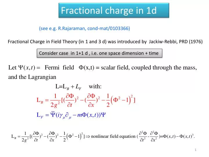
Consider case in 1+1 d , i.e. one space dimension + time Fractional charge in 1d (see e.g. R.Rajaraman, cond-mat/0103366) Fractional Charge in Field Theory (in 1 and 3 d) was introduced by Jackiw-Rebbi, PRD (1976)
Additional static (time-independent) solutions: soliton sector
Dirac’s theory Vacuum sector: field in 1+1 dimensional theory
Electron-Positron field in Dirac’s theory Field in 1+1 dimensional theory
Charge conjugation in 1+1 dimensional theory Charge operator in Dirac’s theory
Positive energy continuum Positive energy continuum localized state negative energy continuum negative energy continuum Soliton sector
Solution in Soliton Sector Solving Dirac’s equation one finds a single 0 mode (solution with E=0). There are two Vacuum states with the zero mode filled or unfilled. These ground states: differ by charge e and are connected by the charge conjugation operator C since H anticommutes with C, therefore the conjugate of a g.s. must be a g.s. with opposite charge. the two ground states must have charge ½ and - ½ .
Fractional Charge in Polyacetilene, Su,Schrieffer and Heeger prl 1979 Unstable vacuum Stable vacuum B Stable vacuum A Soliton
Compare stable vacuum A and vacuum+2 solitons: perturbation is local however solitons can be delocalized:
How many bonds change overall? 7 6 however solitons can be delocalized: It is a matter of 1 electron (per spin) per bond, that is, ½ electron per soliton.
Relation to field theory model The Dirac equation arises by linearizing the energy dispersion near the “Dirac points” which are intersections of the energy dispersion with the Fermi level.
Analogy with field theory model The Dirac equation is in one spatial dimension and involves two components, corresponding to two Dirac points:
Magnetism from Coulomb interactions Magnetism si caused by electrostatic interactions independent of the spin, and is essentially an effect of correlation. But how much do we know the way in which this happens? What causes the antiferromagnetic order in CuO2 and NiO? Much progress has been done by the Hubbard model and related models. The CuO2 antiferromagnetic order Hubbard Model with nearest-neighbor hopping on a lattice L Many interesting resulys are known for bipartite lattices. Bipartite lattice (first neighbors of black sites are red, first neighbors of red sites are black)
Hubbard Model with nearest-neighbor hopping on a lattice L John Hubbard London 1931-San Jose 1980 Many interesting resulys are known for bipartite lattices. Bipartite lattice (first neighbors of black sites are red, first neighbors of red sites are black)
Chain: Bipartite lattices Chain (d=1), square (d=2) , cubic (d=3) lattices 17 17
Bipartite lattice Square lattice
Bipartite lattice Cubic lattice
Spin in Hubbard Model The total spin is conserved. Recalling the general rule for writing operators in second quantization, 20
. Trasformazione a U negativo Possiamo fare una trasformazione canonica sui soli stati di spin su introducendo le buche col che il termine cinetico di spin su diventa A questo punto in un reticolo bipartito possiamo ripristinare il segno cambiando segno a t; questa e’una gauge, perche’ equivale a cambiare di segno gli spinorbitali di un sottoreticolo, 21
Con questo, quando scambiamo creazione e distruzione, solo il termine in U cambia segno: Abbiamo mappato il problema repulsivo e-e in uno attrattivo e-h. Pero’ gli operatori di spin originali una volta espressi in termini e-h cambiano forma: Questi operatori e-e non hanno piu' nel problema attrattivo il significato di spin (si chiamano infatti pseudospin). Essi seguitano ad essere conservati, insieme a quelli e-h di spin. 22
Theorems on Ferromagnetism in Hubbard Model I state without proof some theorems No ferromagnetism at small U. The minimum energy increases with spin. Theorem: Pieri, Daul, Baeriswyl, Dzierzawa, and Fazekas theorem: no ferromagnetism in Hubbard model at very low electron density. 23
Teorema di Lieb-Mattis Phys. Rev. 125, 164 (1962) Consideriamo il modello di Hubbard repulsivo in 1d con obc (open boundary conditions) Gli hoppings (a primi vicini) e gli U possono dipendere dal sito. Sia Emin(S) l’energia dello stato fondamentale con spin S. Allora, con qualsiasi filling, Piu’ basso lo spin piu’ bassa e’ l’energia. Questo e’ ovvio per U=0 quando i livelli si riempiono secondo l’aufbau ma resta vero con U. Quindi non c’e’ ferromagnetismo. L’avevamo visto con il modello di Ising. Niente transizioni di fase in 1d. Rientra nei teoremi di Lieb che dimostreremo piu’ avanti. 24
Strong couplinghalffilledHubbard Model, d=2 or 3 Half filling: number of sites= number of electrons At order 0 in hopping t, there is an electron per site, and huge degeneracy (each spin can be +/-). For 2 sites one has 4 ground states: In first order in t one gets nothing (H takes to doubly occupied states orthogonal to g.s.) isforbidden for infinite U configuration
In second order there are processes where an electron hops from site a with spin + to neighbouring site b (provided that the ground state spin there is -) producing a doubly occupied virtual state (energy U) and back. One can describe that by an effective Hamiltonian: a b Thisisimpossible for parallel spins. Scond-ordercorrections are always negative. So antiparallelconfigurations are lower. 26
Important case: Three-band Hubbard Model of CuO The Cuprates are known to be antiferromagnetsathalffilling. By hole doping (and sometimesalso by electron doping) theybecome high temperature superconductors. In the CuO structure with half filled Cu band this mechanism favors antiferromagnetism. The AF configuration allows the second-order spin exchange. This further lowers the energy. 27
Non-interaction terms linear in n just renormalize all site energies. We ignore them. Besides aba processes one must include bab and all other sites on same footing. Neglecting parallel-spin interactions , part of the physics corresponds to an Hamiltonian of the form sometimes written as:
This model was considered on a bipartite AB lattice in a famous paper by Lieb and Mattis (J. Mathematical Physics 3, 749 (1962)). They were able to show that in the ground state the spin of the elementary cell is 2S=|B|-|A| where |B| and |A| are the numbers of sites in the two lattices. So one can indeed have magnetism. We use this result later. I just mention a related model that P.W. Anderson likes for Cuprate superconductors: the t-J model, appropriate for strong coupling:
Toy Model: 2 electrons on 3 sites (Hal Tasaki , Cond-mat/9512169) for t=t’/2 the ground state has S=1 if U is large (ferro) and S=0 otherwise For t=t’>0 lo stato fondamentale ha S=1 per ogni U (ferro). 30
Perron-Frobenius theorem for real symmetric matrices Proof. Consider the eigenvalue equation Mu=m u. Hence either the components ui have both signs or they must be all strictly positive (or all strictly negative). 31
Pick a vector u having for components the absolute values of those of v, ui=|vi| . We use a variational argument: One cannot change sign to some components without changing the summations (and thus violating the above conclusions) except the case of disconnected clusters that we have excluded by hypothesis. Then v=u (or v=-u, which is the same solution) Then u=v has all strictly positive components. Two ground eigenvectors cannot exist, because they cannot be orthogonal. Then u is the only ground eigenvector . 32
Nagaoka’s saturated Ferromagnetism Y. Nagaoka’s Theorem (weak version) Consider a Hubbard Model with infinite U on any lattice L in d=2 and in d=3 with (possibly long range ) non negative hopping t. Let Ne=| L |-1 , that is, the electron number is the number of sites minus 1. Then among the ground states there are some with maximal spin (Ne/2). Informal Proof In the infinite U limit the Hilbert space consists of the configurations with no double occupation. An orthogonal basis for such an Hilbert space can be specified by assigning the position x of the hole in the lattice and the spin configuration on all the other sites. Just for notational simplicity I exemplify by this 5-atom cluster. The basis vectors with the hole in 1 are: We need the action of the hopping Hamiltonian on this: for instance the matrix element: 33
We must choose the spin configuration that gives maximum hopping and therefore maximum band width and lowest minimum energy. It is clear that by taking all spins parallel the delta is always satisfied and if we look for the ground state among parallel spin configurations we do find a lower ground state. A more formal proof reaches this conclusion by the Schwartz inequality, but this is the essential reason. Details are in Hal Tasaki cond-mat/9712219
Nagaoka Y. Nagaoka’s Theorem (strong version) Consider a Hubbard Model with infinite U on any lattice L in d=2 and in d=3 with (possibly long range ) non negative hopping t. Let Ne=| L |-1 , that is, the electron number is the number of sites minus 1. Assume that the connectivity condition is satisfied. Then the ground states has maximal spin (Ne/2) and has no other degeneracy. Informal Proof All the matrix elements like are negative if both states. The Perron-Frobenius theorem implies that the ground state in the space with a fixed total Sz is unique. The connectivity condition which is required by Frobenius holds for all common lattices. The theorem showed for the first time that dtrong correlation can lead to ferromagnetism. Remark At half filling there is no ferromagnetism. This theorem is surprising and cannot be understood in terms of mean field! 35