Download
1 / 61
610 likes | 775 Vues
On the use of statistical tools for audio processing. Mathieu Lagrange and Juan José Burred Analyse / Synthèse Team, IRCAM Mathieu.lagrange@ircam.fr. École centrale de Nantes Filière ISBA . Outline . Introduction Context and challenges Past and Present Speech Model

E N D
On the use of statistical tools for audio processing • Mathieu Lagrange and Juan José Burred • Analyse / Synthèse Team, IRCAM • Mathieu.lagrange@ircam.fr École centrale de Nantes Filière ISBA
Outline • Introduction • Context and challenges • Past and Present • Speech • Model • Applications (coding, speaker recognition, speech recognition) • Audio (Music) • Sound models • Applications (classification, similarity) • Limitations • Sound source separation • Paradigms, tasks and applications • Mixing Models • Methods for the under determined case • Clustering of Spectral Audio (CoSA) • Auditory Scene Analysis (ASA) • Clustering
Outline • Introduction • Context and challenges
Technological Context « We are drowning in information and starving for knowledge » R. Roger • Needs: • Measurement • Transmission • Access • Aim of a numerical representation: • Precision • Efficiency • Relevance • Means • Mechanical biology • Psycho-acoustic • Cognition
Challenges « Forty-two! yelled Loonquawl. Is that all you've got to show for seven and a half million years' work? » D. Adams Music is great to study as it is both: • object : arrangement de sons et de silences au cours du temps • function: more or less codified form of expression of : • Individual feelings (mood) • Collective feelings (party, singing, dance)
Outline • Introduction • Context and challenges • Past and Present • Speech • Model • Applications (coding, speaker recognition, speech recognition)
Speech signal • The speech signal is produced when the air flow coming from the lungs go through the vocal chords and the vocal tract. • The size and the shape of the vocal tract as well as the vocal chords excitations are changing relatively slowly • The speech signal can therefore be considered as quasi-stationary over short period of about 20 ms. • Type of speech production • Voiced: <a>, <e>, … • Unvoiced: <s>, <ch>, • Plosives: <pe>, <ke>
Source / Filter Model • In the case of an idealized voiced speech signal, the vocal chords are producing a perfectly periodic harmonic signal • The influence of the vocal tract can be considered as a filtering with a given frequency response whose maximas are called formants.
Source / Filter Coding • Algorithm : • Voiced / Unvoiced detection; • Voiced case: the source signal is approximated with a Dirac comb: • a Dirac comb whose successive Diracs are respectively T spaced by T as a spectrum which is a Dirac comb whose successive combs are 1/T spaced. • Parameters : T, gain • Unvoiced: the source signal is approximated by a stochastic signal: • Parameter : gain. • The Source signal is next filtered. • Parameters : filter coefficients.
« Code-Excited Linear Predictive » (CELP) For each frame of 20 ms : • Auto-Regressive coefficients are computed such that the prediction error is minimized over the entire duration of the frame: • Quantified coefficients and an index encoding the error signal are transmitted.
« Code-Excited Linear Predictive » (CELP) index Residual AR Coefficients Signal
Speaker Recognition • Classical pattern recognition problem • Specific problems: • Open Set / Closed Set: rejection problem • Identification / Verification • Text Dependency • Method • Feature extraction: model each speech with Mel-Frequency Cepstral Coefficients (MFCCs) and their derivatives. • Classification • Text independent: Vector Quantization Codebooks or Gaussian Mixture Models (GMMs) • Text dependent: Dynamic Time Warping (DTW) or Hidden Markov Model (HMM) s1 s2 s3
Speech recognition • An Automatic Speech Recognition System is typically decomposed into: • Feature Extraction: MFCCs • Acoustic Models: HMMs trained for set of phones • Each phone is modelled with 3 states • Pronunciation dictionary: convert a series of phones into a word • Language Model: predict the likelihood of specific words occurring one after another with n-grams (Fig. from HTK documentation)
MFCCs rules ? Mel Frequency Cepstral Coefficients are commonly derived as follows: • Take the Fourier transform of (a windowed excerpt of) a signal. • Map the powers of the spectrum obtained above onto the mel scale, using triangular overlapping windows. • Take the logs of the powers at each of the mel frequencies. • Take the discrete cosine transform (DCT) of the list of mel log powers, as if it were a signal. • The MFCCs are the amplitudes of the resulting spectrum.
Issues with MFCCs computation steps • The MEL frequency wraping: • highly criticized form a perceptual point of view (Greenwood) • conceptually: periodicity analysis over data that are not periodic anymore (Camacho) • The Cepstral Coefficients are COSINE coefficients: • cannot shift with speaker size to capture the shift in formant frequencies that occurs as children grow up and their vocal tracts get longer • Not a sound representation: • no way to provide enhancements such as speaker and channel adaptation, background noise suppression, source separation
Potentials of the DCT step • Observation of Pols that the main components capture most of the variance using a few smooth basis functions, smoothing away the pitch ripples • Principal components of a collection of vowel spectra on a warped frequency scale aren't so far from the cosine basis functions • Decorrelates the features. • This is important because the MFCC are in most cases modelled by Gaussians with diagonal covariance matrices
Outline • Introduction • Context and challenges • Past and Present • Speech • Model • Applications (coding, speaker recognition, speech recognition) • Audio (Music) • Sound models • Applications (classification, similarity) • Limitations
Sound Models • Major classes of sounds • Transients (castanets, …) • Pseudo periodic (flute, …) • Stochastic (waves, …) • Models • Impulsive noise • Sum of sinusoids • Wide band noise
Classification • Method: [Tzanetakis’02] • Agree on mutually exclusive set of tags (the ontology) • Extract features from audio (MFCCs and variations) • Train statistical models: • Due to the high dimensionality of the feature vectors discriminatives approaches are prefered (SVMs) • Segmentation • Smoothing decision using dynamic programming (DP) (Fig. from [Ramona07])
Multi-Class Discriminative Classification • Usually performed by combining binary classifiers • Two approaches: • One-vs-all: For each class build a classifier for that class versus the rest • Often very imbalanced classifiers (use asymmetric regularization) • All-vs-all Build a classifier for each couple of class • A priori a large number of classifiers to build but the pairwise classification are faster and the classifications are balanced (easier to find the best regularization) s1 s2 s3
Multi-Label Discriminative Classification • Each object may be tagged using several labels • Computational approaches • Power Sets • Binary Relevance (equivalent to one-vs-all) • Multiple criteria: • « Flattening » the ontology • Research trend: considering the ontology structure to benefit from co-occurrence labels of different semantic criterion C2 C1 C3
Music Similarity • Question to solve: « Given a seed song, provide us with the entries of the database which are the most similar » • Annotation type: Artist / Album • Method: [Aucouturier’04] • Songs are modeled as GMM of MFCCs • Proximity of GMMs are considered as similiarity measure: • Likelihood (requires access to the MFCCs) • Sampling
Cover Version Detection • Question to solve: « Given a seed song, provide us with the entries of the database which are cover versions » • Annotation: canonical song • Method: [Serra’08] • Songs are modeled as a time series of Chromas • Computation of the similarity matrix between the two time series • Similarity is measured using Dynamic Programming Local Alignment (Fig. from [Serr08])
Limitations • Description of audio and music • Polyphonic • Multiple shapes varying in various ways • Statistical Modeling • Curse of dimensionality • Sense of structure relevant at multiple levels of temporality
Outline • Introduction • Context and challenges • Past and Present • Speech • Model • Applications (coding, speaker recognition, speech recognition) • Audio (Music) • Sound models • Applications (classification, similarity) • Limitations • Sound source separation • Paradigms, tasks and applications • Mixing Models • Methods for the under determined case
Sound Source Separation • “Cocktail party effect” • E. C. Cherry, 1953. • Ability to concentrate attention on a specific sound source from within a mixture. • Even when interfering energy is close to energy of desired source. • “Prince Shotoku Challenge” • Legendary Japanese prince Shotoku (6th Century AD) could listen and understand simultaneously the petitions by ten people. • Concentrate attention on several sources at the same time! • “Prince Shotoku Computer” (Okuno et al., 1997) • Both allegories imply an extra step of semantic understanding of the sources, beyond mere acoustical isolation.
The paradigms of Musical Source Separation • (based on [Scheirer00]) • Understanding without separation • E.g. music genre classification • “Glass ceiling” of traditional methods (MFCC+GMM) [Aucouturier&Pachet04] • Separation for understanding • First (partially) separate, then feature extraction • Source separation as a way to break the glass ceiling? • Separation without understanding • BSS: Blind Source Separation (ICA, ISA, NMF) • Blind means: only very general statistical assumptions taken. • Understanding for separation • Supervised source separation (based on a training database)
Required sound quality • Audio Quality Oriented (AQO) • Aimed at full unmixing at the highest possible quality. • Applications: • Unmixing, remixing, upmixing • Hearing aids • Post-production • Significance Oriented (SO) • Separation quality just enough for facilitating semantic analysis of complex signals. • Less demanding, more realistic. • Applications: • Music Information Retrieval • Polyphonic Transcription • Object-based audio coding
Musical Source Separation Tasks • Classification according to the nature of the mixtures: • Classification according to available a priori information:
Linear mixing model • Only amplitude scaling before mixing (summing) • Linear stereo recording setups: XY Stereo MS Stereo Close miking Direct injection
Delayed mixing model • Amplitude scaling and delay before mixing • Delayed stereo recording setups: Close miking with delay Direct injection with delay AB Stereo Mixed Stereo
Convolutive mixing model • Filtering between sources and sensors • Convolutive stereo recording setups: Close miking with reverb Direct injection with reverb Reverberant environment Binaural
Some terminology • System of linear equations: • Usual algebraic methods from high school: X known, A known, S unknown • But in source separation: unknown variables (S, sources) AND unknown coefficients (A, mixing matrix) • Algebra terminology is retained for source separation: • More equations (mixtures) than unknowns (sources): overdetermined • Same number of equations (mixtures) than unknowns (sources): determined (square A) • Less equations (mixtures) than unknowns (sources): underdetermined • The underdetermined case is the most demanding, but also the most important for music! • Music is (still) mostly in stereo, with usually more than 2 instruments • Overdetermined and determined situtations are only of interest for arrays of sensors or arrays of microphones (localization, tracking)
Binaural Case (1) • Goal: find a mask M that retrieves one source when used to filter a given time-frequency representation. • DUET (Degenerate Unmixing Estimation Technique) [Yilmaz&Rickard04] • Histogram of Interchannel Intensity (IID) and Phase (IPD) Differences • Binary Mask created by selecting bins around histogram peaks. • Drawback of t-f masking: “musical noise” or “burbling” artifacts º is the Hadamard (element-wise) product (Fig. from [Vincent06]) (Fig. from [Yilmaz&Rickard04])
Binaural Case (2) • Human-assisted time-frequency masking[Vinyes06] • Human-assisted selection of the time-frequency bins out of the DUET-like histogram for creating the unmixing mask • Implementation as a VST plugin (“Audio Scanner”)
Monaural Case • Classification according to a priori knowledge • Supervised • Based on training the model with a sound example database • Better quality and more demanding situations at the cost of less generality • Unsupervised • Classification according to model type • Adaptive basis decompositions (ISA, NMF, NSC) • Sinusoidal Modeling • Classification according to mixture type • Monaural systems • Hybrid systems combining advanced source models with spatial diversity
Independent Subspace Analysis • Application of ISA to audio: Casey and Westner, 2000. • Application of ICA to the spectogram of a mono mixture. • Each independent component corresponds to an independent subspace of the spectrogram. (Fig. from [Casey&Westner00]) • Component-to-source clustering • The extracted components usually do not directly correspond to the sources. • They must be clustered together according to some similarity criterion. • Casey&Westner use a matrix of Kullback-Leibler divergences called the ixegram.
ICA for Audio (Figs from Virtanen)
Nonnegative Matrix Factorization • Matrix factorization ( ) imposing non-negativity. • Needed when using magnitude or power spectrograms. • NMF does not aim at statistical independence, but: • It has been proven that, under some conditions, non-negativity is sufficient for separation. • NMF yields components that very closely correspond to the sources. • To date, there is no exact theoretical explanation why is that so! • Use for transcription: • P. Smaragdis and J.C. Brown. Non-Negative Matrix Factorization for Polyphonic Music Transcription. Proc. IEEE Workshop on Applications of Signal Processing to Audio and Acoustics (WASPAA), New Paltz, USA, 2003. • Use for separation: • B. Wang and M. D. Plumbley. Musical Audio Stream Separation by Non-Negative Matrix Factorization. Proc. UK Digital Music Research Network (DMRN) Summer Conf., 2005.
NMF for Audio (Figs from Virtanen)
NMF for Vision • By representing signals as a sum purely additive, non- negative sources, we get a parts-based representation [Lee’99]
Mixture Component 1 Component 2 Mixture Component 1 Component 2 Nonnegative Sparse Coding • Combination of non-negativity and sparsity constraints in the factorization. • [Virtanen03]: NSC is optimized with an additional criterion of temporal continuity. • Measured by the absolute value of the overall amplitude difference between consecutive frames. • [Virtanen04]: Convolutive Sparse Coding • Improved temporal accuracy by modeling the sources as the convolution of spectrograms with a vector of onsets.
Separated sources Mixture Sinusoidal Methods • Sinusoidal Modeling: detection and tracking of the sinusoidal partial peaks on the spectrogram. • Based on Auditory Scene Analysis (ASA) cues of good-continuation, common fate and smoothness of sinusoidal tracks. • Overall, very good reduction of interfering sources, but moderate timbral quality. • Appropriate for Significance-Oriented applications • [Virtanen&Klapuri02]: model of spectral smoothness of harmonic sounds • Based on basis decomposition of harmonic structures • Additive resynthesis of partial parameters • [Every&Szymanski06] • Spectral subtraction instead of additive resynthesis (Fig. from [Every06])
Separation of chords Inharmonic separation Mixture Separated sources Mixture Separated sources Supervised Methods (1) • Use of a training database to create a set of source models, each one modeling a specific instrument. • Better separation as a trade-off for generality. • Supervised sinusoidal methods • [Burred&Sikora07] • The source models are compact descriptions of the spectral envelope and its temporal evolution. • The detailed temporal evolution allows to ignore harmonicity constraints, and thus separation of chords and inharmonic sounds is possible.
Separated sources Mixture Separated sources Mixture Supervised Methods (2) • Bayesian Networks • [Vincent06] • Multilayered model describing note probabilities (state layer), spectral decomposition (source layer) and spatial information (mixture layer). • Trained on a database of isolated notes. • Allows separation of sounds with reverb. • Learnt priors for Wiener-based separation • [Ozerov05] • Single-channel • GMM models of singing voice and accompaniment.
Conclusions • Still far from fully-general, audio-quality-oriented system. • More realistic: significance oriented • Separation good enough to facilitate content analysis • Methods based on adaptive models, time-frequency masking: • More realistic mixtures, but more artifacts and interferences • Methods based on sinusoidal modeling: • More artificial timbre, but less interferences. • Current polyphony limitations: • Mono signals: up to 3, 4 instruments • Stereo signals: up to 5, 6 instruments
Outline • Introduction • Context and challenges • Past and Present • Speech • Model • Applications (coding, speaker recognition, speech recognition) • Audio (Music) • Sound models • Applications (classification, similarity) • Limitations • Sound source separation • Paradigms, tasks and applications • Mixing Models • Methods for the under determined case • Clustering of Spectral Audio (CoSA) • Auditory Scene Analysis (ASA) • Clustering
Binary Masking with Oracle • Binary masking is an effective way of performing the separation • Using an oracle allows to assess the relevance of Fourier spectrograms as an atomic representation • The binary mask is set to 1 if the source of interest is dominant in the considered frequency bin, and 0 otherwise STFT ISTFT |STFT| Mask