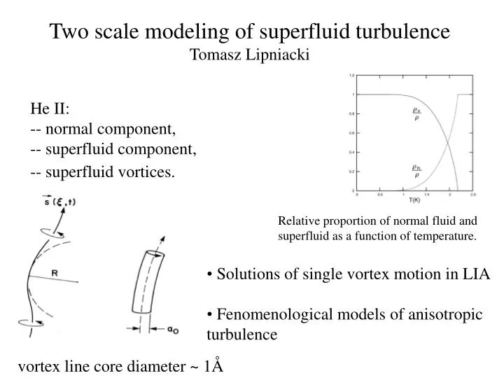
Two scale modeling of superfluid turbulence Tomasz Lipniacki

1. Two scale modeling of superfluid turbulence Tomasz Lipniacki He II: -- normal component, -- superfluid component, -- superfluid vortices. Relative proportion of normal fluid and superfluid as a function of temperature. • Solutions of single vortex motion in LIA • Fenomenological models of anisotropic • turbulence vortex line core diameter ~ 1Å

2. Localized Induction Approximation c - curvature - torsion

3. Ideal vortex Totally integrable, equivalent to non-linear Schrödinger equation. Countable (infinite) family of invariants: Quasi static solutions:

4. Hasimoto soliton on ideal vortex (1972) : F i g u r e 1 2

5. Kida 1981 General solutions of in terms of elliptic integrals including shapes such as circular vortex ring helicoidal and toroidal filament plane sinusoidal filament Euler’s elastica Hasimoto soliton

6. Quasi static solutions for quantum vortices ? Quantum vortex shrinks:

7. Quasi-static solutions Lipniacki JFM2003 Frenet Seret equations

8. In the case of pure translation we get analytic solution For where Solution has no self-crossings

9. Quasi-static solution: pure rotation Vortex asymptotically wraps over cones with opening angle for in cylindrical coordinates where

10. Quasi-static solution: general case For vortex wraps over paraboloids

11. Results in general case I. 4-parametric class of solutions, determined by initial condition II. Each solution corresponds to a specific isometric transformation G(t)related analytically to initial condition. III. The asymptotic for is related analytically via transformation G(t) to initial condition.

12. Shape-preserving solutions Lipniacki, Phys. Fluids. 2003 Equation is invariant under the transformation If the initial condition is scale-free, than the solution is self-similar In general scale-free curve is a sum of two logarithmic spirals on coaxial cones; there is four parametric class of such curves.

13. Shape-preserving solutions • solutions with decreasing scale

14. Analytic result: shape-preserving solution In the case when transformation is a pure homothety we get analytic solution in implicit form:

15. Shape preserving solution: general case Logarithmic spirals on cones

16. Results in general case I. 4-parametric class of solutions, determined by initial condition II. Each solution corresponds to a specific similarity transformation III. The asymptotics for is given the initial condition of the original problem (with time).

17. Self-similar solution for vortex in Navier-Stokes? N-S is invariant to the same transformation The friction coefficient corresponds to

18. Wing tip vortices

19. Macroscopic description -- Euler equation for superfluid component -- Navier-Stokes equation for normal component Coupled by mutual friction force where and L is superfluid vortex line density.

20. Microscopic description of tangle superfluid vortices Aim Assuming that quantum tangle is “close” to statistical equilibrium derive equations for quantum line length density L and anisotropy parameters of the tangle. Statistical equilibrium? Two cases I – rapidly changing counterflow, but uniform in space II – slowly changing counterflow, not uniform in space

21. Model of quantum tangle “Particles” = segments of vortex line of length equal to characteristic radius of curvature. Particles are characterized by their tangent t, normal n, and binormal b vectors. Velocity of each particle is proportional to its binormal (+collective motion). Interactions of particles = reconnections.

22. Reconnections 1. Lines lost their identity: two line segments are replaced by two new line segments 2. Introduce new curvature to the system 3. Remove line-length

23. Motion of vortex line in the presence of counterflow Evolution of its line-length is

24. Evolution of line length density where average curvature average curvature squared Average binormal vector (normalized) I

25. Rapidly changing counterflow Generation term: polarization of a tangle by counterflow Degradation term: relaxation due to reconnections

26. Generation term: polarization of a tangle by counterflow evolution of vortex ring of radius R and orientation in uniform counterflow unit binormal Statistical equilibrium assumption: distribution of f(b) is the most probable distribution giving right I i.e.

27. Degradation term: relaxation due to reconnections Reconnections produce curvature but not net binormal Total curvature of the tangle Reconnection frequency Relaxation time:

28. Finally Lipniacki PRB 2001

29. Model prediction: there exists a critical frequency of counterflow above which tangle may not be sustained

30. Quantum turbulence with high net macroscopic vorticity Vinen-Schwarz equation We assume now Let denote anisotropy of the tangent Vinen type equation for turbulence with net macroscopic vorticity

31. Drift velocity where

32. Mutual friction force drag force where finally

33. Helium II dynamical equations Lipniacki EJM 2006

34. Specific cases: stationary rotating turbulence Pure heat driven turbulence Pure rotation „Sum” Fast rotation Slow rotation

35. Plane Couette flow V- normal velocity U-superfluid velocity q- anisotropy l-line length density

36. “Hypothetical” vortex configuration

37. Summary and Conclusions • Self-similar solutions of quantum vortex motion in LIA • Dynamic of a quantum tangle in rapidly varying counterflow • Dynamic of He II in quasi laminar case. • In small scale quantum turbulence, the anisotropy of • the tangle in addition to its density L is key to analyze • dynamic of both components.

39. Non-linear Schrodinger equation (Gross, Pitaevskii) For Madelung Transformation superfluid velocity superfluid density

40. Modified Euler equation With pressure Quantum stress

41. Mixed turbulence Kolgomorov spectrum for each fluid - energy flux per unit mass

44. Two scale modeling of superfluid turbulence Tomasz Lipniacki He II: -- normal component, -- superfluid component, -- superfluid vortices. Relative proportion of normal fluid and superfluid as a function of temperature. vortex line