Download

1 / 52
520 likes | 532 Vues
CS 5224 High Speed Networks and Multimedia Networking. Dr. Chan Mun Choon Semester 1, 2005/2006 School of Computing National University of Singapore. Organization. Lecturer: Dr. Chan Mun Choon ( chanmc@comp.nus.edu.sg ) Homepage: http://www.comp.nus.edu.sg/~chanmc Office: S14 #06-09

E N D
CS 5224High Speed Networks and Multimedia Networking Dr. Chan Mun Choon Semester 1, 2005/2006 School of Computing National University of Singapore
Organization • Lecturer: • Dr. Chan Mun Choon (chanmc@comp.nus.edu.sg) • Homepage: http://www.comp.nus.edu.sg/~chanmc • Office: S14 #06-09 • Tel: 6874-7372 • Course Information • Web-site: http://www.comp.nus.edu.sg/~cs5224 • IVLE • Class Venue: S16 #04-05 (SR1) • Class Time: 6:30pm – 8:30pm, Wednesday • Office Hours: 3:30pm – 5:30pm Wednesday Introduction/Basic Concept
Course Description • Introduce graduate students to fundamental networking problems and concepts • For students interested in the area of networking, this course will be rewarding • Emphasis on problem solving and performance evaluation (queuing theory, graph algorithms etc.) • Long homework • Midterm + Finals Introduction/Basic Concept
Course Pre-requisites • Assume students have taken undergraduate networking classes like CS2105/CS3103 • Basic background on probability and algorithms • Textbooks: • S. Keshav, "An Engineering Approach to Computer Networking", Addison-Wesley. • Reference Books • Bertsekas and Gallager, "Data Networks", 2nd Edition, Prentice Hall Introduction/Basic Concept
(Tentative) Outline/Schedule 1 10/8 Introduction and basic concepts 2 17/8 Multiplexing, Queuing Theory 3 24/8 Traffic Engineering (HW1 Assign) 4 31/8 Simulation (HW1 Due) 5 7/9 Scheduling and Buffer Management (Hw 2 Assign) 6 14/9 Scheduling and Buffer Management (HW 2 Due) 21/8 Mid-Semester Break 7 28/9 Midterm Exam 8 5/10 Routing 9 12/10 Routing (HW3 Assign) 10 19/10 End-to-end Performance (HW3 Due) 11 26/10 Transport 12 2/11 Wireless Networks (HW4 Assign) 13 9/11 Access/High Speed Networks 16/11 Reading Day (HW 4 Due) Introduction/Basic Concept
(Tentative) Grading Policy • Homework 35% (4 Assignments) • Class Participation 5% • Mid-Term Exam 25% • Final Exam 35% Introduction/Basic Concept
Outline • Types of Communication Networks • Quality of Service Measure and Classes • Design issues/principles Introduction/Basic Concept
Speed and Distance of Communications Networks Introduction/Basic Concept
Characteristics of WANs • Covers large geographical areas • Circuits provided by a common carrier • Consists of interconnected switching nodes • Legacy WANs provide modest connection capacity • 64 kbps were common • Business subscribers uses T1 (1.544Mbps) • Current WAN connections • Higher-speed WANs use optical fiber and transmission technique known as asynchronous transfer mode (ATM) or SONET • T1/DS3(45Mbps)/OC3(155Mbps)/OC12, Ethernet • 10, 100 of Mbps or more are common Introduction/Basic Concept
Characteristics of LANs • Like WAN, LAN interconnects a variety of devices and provides a means for information exchange among them • Legacy LANs • Provide data rates of 1 to 20 Mbps • High-speed LANS • Provide data rates of 100 Mbps to 10 Gbps Introduction/Basic Concept
Switching Terms • Switching Nodes: • Intermediate switching device that moves data • Not concerned with content/payload of data • Switch based on timing or header information • Stations: • End devices that wish to communicate • Each station is connected to a switching node • Communications Network: • A collection of switching nodes Introduction/Basic Concept
Switched Network Introduction/Basic Concept
Observations of Figure 3.3 • Some nodes connect only to other nodes (e.g., 5 and 7) • Some nodes connect to one or more stations • Node-station links usually dedicated point-to-point links • Node-node links usually multiplexed links • Shared among difference source-destination pairs • Not a direct link between every node pair • Directly connecting all pairs requires N(N-1) or O(N2) links Introduction/Basic Concept
Techniques Used in Switched Networks • Circuit switching • Dedicated communications path between two stations • E.g., public telephone network • Packet switching • Message is broken into a series of packets • Each node determines next leg of transmission for each packet Introduction/Basic Concept
Phases of Circuit Switching • Circuit establishment • An end to end circuit is established through switching nodes • Information Transfer • Information transmitted through the network • Data may be analog voice, digitized voice, or binary data • Circuit disconnect • Circuit is terminated • Each node deallocates dedicated resources Introduction/Basic Concept
Characteristics of Circuit Switching • Can be inefficient • Channel capacity dedicated for duration of connection • Utilization not 100% • Delay prior to signal transfer for establishment • Once established, network is transparent to users • Information transmitted at fixed data rate with only (fixed) propagation delay • Best known circuit switched network is the Public Switch Telephone Network (PSTN) Introduction/Basic Concept
How Packet Switching Works • Data is transmitted in blocks, called packets • Before sending, the message is broken into a series of packets • Packets consists of a portion of data plus a packet header that includes control information • At each node en route, packet is received, stored briefly and passed to the next node • The store and forward mode of operation incurred both (variable) queuing delay and propagation delay Introduction/Basic Concept
Packet Switching Introduction/Basic Concept
Packet Switching Advantages • Line efficiency is greater • Many packets over time can dynamically share the same node to node link • Packet-switching networks can carry out data-rate conversion • Two stations with different data rates can exchange information • Unlike circuit-switching networks that block calls when traffic is heavy, packet-switching still accepts packets, but with increased delivery delay • Priorities can be used at the packet level Introduction/Basic Concept
Disadvantages of Packet Switching • Each packet switching node introduces a delay • Overall packet delay can vary substantially • This is referred to as jitter • Caused by differing packet sizes, routes taken and varying delay in the switches • Each packet requires overhead information • Includes destination and sequencing information • Reduces communication capacity • More processing required at each node Introduction/Basic Concept
Packet Switching Networks - Virtual Circuit • Preplanned route established before packets sent • All packets between source and destination follow this route • Routing decision not required by nodes for each packet • Emulates a circuit in a circuit switching network but is not a dedicated path • Packets still buffered at each node and queued for output over a line Introduction/Basic Concept
Packet Switching Networks – Virtual Circuit • Advantages: • Packets arrive in original order • Packets arrive correctly • Packets transmitted more rapidly without routing decisions made at each node • This is how ATM network works Introduction/Basic Concept
Packet Switching Networks - Datagram • Each packet treated independently, without reference to previous packets • Each node chooses next node on packet’s path • Packets don’t necessarily follow same route and may arrive out of sequence • Exit node restores packets to original order • Responsibility of exit node or destination to detect loss of packet and how to recover Introduction/Basic Concept
Packet Switching Networks – Datagram • Advantages: • Call setup phase is avoided • Because it’s more primitive, it’s more flexible • Datagram delivery is more “reliable” • This is how the Internet works Introduction/Basic Concept
Example • Imagine a postal system implemented in the following ways: • 1. All mails coming from zip code 123456 will be delivered to 654321. This is ____________ • 2. The zip code of all mails coming from zip code 123456 will be changed to 654321 and sent to the post office in Kent Ridge. This is ____________ • 3. The zip code of all mails coming from zip code 123456 will be delivered to Kent Ridge. This is ____________ Introduction/Basic Concept
Networking modes Switching modes Connection-oriented Connectionless Packet-switching Circuit-switching Recap: different types of networks • A network is defined by its “switching mode” and its “networking mode” • Circuit switching vs. packet switching • Circuit-switching: switching based on position (space, time, ) of arriving bits • Packet-switching: switching based on information in packet headers • Connectionless vs. connection-oriented networking: • CL: Packets routed based on address information in headers • CO: Connection set up (resources reserved) prior to data transfer MPLS IP + RSVP ATM, X.25 IP, SS7 Telephone network, SONET/SDH, WDM Introduction/Basic Concept
Consuming end Stored Live Sending end Live Stored Types of data transfers • An application could consist of different types of data transfers • An http session has an interactive component, but could also have a non-real-time transfer Interactive/ Live streaming Recording Stored streaming File transfers Introduction/Basic Concept
Non-real-time (stored at sender and receiver ends) Real-time (consumed or sent live) Interactive (two-way) (consumed/sent live) e.g. telephony, on-line interactive games Streaming (one-way) (consumed live; sent from live or stored source) e.g. radio/TV broadcasts Short transfers (e.g. short email) Long transfers (e.g. large image, audio, video or data) Recording (one-way) (stored at receiver end; sent from live source); e.g. Replay Interactive (two-way) (consumed/sent live) e.g. telnet, http, games Matching applications & networks Data transfers Circuit-switched networks Connectionless networks Packet-switched CO networks Introduction/Basic Concept
Outline • Types of Communication Networks • Quality of Service Measure and Classes • Design issues and Scalability Requirements of Networks Introduction/Basic Concept
“Quality of Service” Measure • How is level of service measured in the network? • Measure can be deterministic or statistical • Common parameters are • bandwidth • delay • delay-jitter • loss Introduction/Basic Concept
Bandwidth • Specified as minimum bandwidth measured over a pre-specified interval • E.g. > 5Mbps over intervals of > 1 sec • Meaningless without an interval! • Can be a bound on average (sustained) rate or peak rate • Peak is measured over a ‘small’ inteval • Average is asymptote as intervals increase without bound Introduction/Basic Concept
Packet Loss • Specified ratio of packet loss over some interval • Like bandwidth, meaningless without some reference to a measurement interval • Common to use an average loss rate measured over a “sufficiently long” interval • Consecutive packet loss can be of interest to some applications, e.g. those with error-correction capability Introduction/Basic Concept
Delay and delay-jitter • Bound on some parameter of the delay distribution curve Introduction/Basic Concept
Packets queue in router buffers packet arrival rate to link exceeds output link capacity packets queue, wait for turn packet being transmitted (delay) packets queueing (delay) free (available) buffers: arriving packets dropped (loss) if no free buffers How do loss and delay occur? A B Introduction/Basic Concept
1. nodal processing: check bit errors determine output link transmission A propagation B nodal processing queueing Four sources of packet delay • 2. queueing • time waiting at output link for transmission • depends on congestion level of router Introduction/Basic Concept
3. Transmission delay: R=link bandwidth (bps) L=packet length (bits) time to send bits into link = L/R 4. Propagation delay: d = length of physical link s = propagation speed in medium (~2x10⁸ m/sec) propagation delay = d/s transmission A propagation B nodal processing queueing Delay in packet-switched networks Note: s and R are very different quantities! Introduction/Basic Concept
Nodal delay • dproc = processing delay • typically a few microsecs or less • dqueue = queuing delay • depends on congestion • dtrans = transmission delay • = L/R, significant for low-speed links • dprop = propagation delay • a few microsecs to hundreds of msecs Introduction/Basic Concept
R=link bandwidth (bps) L=packet length (bits) a=average packet arrival rate Queueing delay (revisited) traffic intensity = La/R • La/R ~ 0: average queueing delay small • La/R -> 1: delays become large • La/R > 1: more “work” arriving than can be serviced, average delay infinite! Introduction/Basic Concept
Packet loss • queue (aka buffer) preceding link in buffer has finite capacity • when packet arrives to full queue, packet is dropped (aka lost) • lost packet may be retransmitted by previous node, by source end system, or not retransmitted at all Introduction/Basic Concept
Outline • Types of Communication Networks • Quality of Service Measure and Classes • Design issues/principles Introduction/Basic Concept
Common design techniques • Key concept: bottleneck • the most constrained element in a system • System performance improves by removing bottleneck • but creates new bottlenecks • In a balanced system, all resources are simultaneously bottlenecked • this is optimal • but nearly impossible to achieve • in practice, bottlenecks move from one part of the system to another Introduction/Basic Concept
Top level goal • Use unconstrained resources to alleviate bottleneck • How to do this? • Several standard techniques allow us to trade off one resource for another Introduction/Basic Concept
Multiplexing • Another word for sharing • Trades time and space for money • Users see an increased response time, and take up space when waiting, but the system costs less • economies of scale Introduction/Basic Concept
Multiplexing (contd.) • Examples • multiplexed links • shared memory • Another way to look at a shared resource • unshared virtual resource • Server controls access to the shared resource • uses a schedule to resolve contention • choice of scheduling critical in proving quality of service guarantees Introduction/Basic Concept
Statistical multiplexing • Suppose resource has capacity C • Shared by N identical tasks • Each task requires capacity c • If Nc <= C, then the resource is underloaded • If at most 10% of tasks active, then C >= Nc/10 is enough • we have used statistical knowledge of users to reduce system cost • this is statistical multiplexing gain Introduction/Basic Concept
Statistical multiplexing (contd.) • Two types: spatial and temporal • Spatial • we expect only a fraction of tasks to be simultaneously active • Temporal • we expect a task to be active only part of the time • e.g silence periods during a voice call Introduction/Basic Concept
Example of statistical multiplexing gain • Consider a 100 room hotel • How many external phone lines does it need? • each line costs money to install and rent • tradeoff • What if a voice call is active only 40% of the time? • can get both spatial and temporal statistical multiplexing gain • but only in a packet-switched network (why?) • Remember • to get SMG, we need good statistics! • Will cover statistical multiplexing in more detail in the queuing theory section Introduction/Basic Concept
Optimizing the common case • 80/20 rule • 80% of the time is spent in 20% of the code • Optimize the 20% that counts • need to measure first! • RISC • How much does it help? • Amdahl’s law • Execution time after improvement = (execution affected by improvement / amount of improvement) + execution unaffected • beyond a point, speeding up the common case doesn’t help Introduction/Basic Concept
Hierarchy • Recursive decomposition of a system into smaller pieces that depend only on parent for proper execution • No single point of control • Highly scaleable • Leaf-to-leaf communication can be expensive • shortcuts help • Most network naming schemes are hierarchical Introduction/Basic Concept