Download
1 / 20
200 likes | 325 Vues
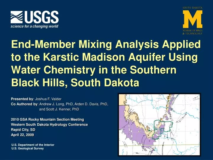
End-Member Mixing Analysis Applied to the Karstic Madison Aquifer Using Water Chemistry in the Southern Black Hills, South Dakota. Presented by : Joshua F. Valder Co Authored by : Andrew J. Long, PhD, Arden D. Davis, PhD, and Scott J. Kenner, PhD

E N D
End-Member Mixing Analysis Applied to the Karstic Madison Aquifer Using Water Chemistry in the Southern Black Hills, South Dakota Presented by: Joshua F. Valder Co Authored by: Andrew J. Long, PhD, Arden D. Davis, PhD, and Scott J. Kenner, PhD 2010 GSA Rocky Mountain Section Meeting Western South Dakota Hydrology Conference Rapid City, SD April 22, 2009
Purpose of the Study • Develop a multivariate statistical approach that can characterize potential sourceareas and mixing proportions. • Sources are not well understood • Mixing proportions are not well understood • Application to chemical data
Location and Scope of the Wind Cave Study • Samples collected during April, May, and July of 2007 • 19 sites • Springs • Sinking Streams • Cave Waters • Wells • 10 species • Ca, Mg, Na+K, SO4, HCO3+CO3, Cl, N, Si, δ2H, δO18 General Direction of Flow
Development of the Approach Three main ideas: (1) Principal Component Analysis and Cluster Analysis, (2) the Conceptual Model, and (3) the MIX Model.
Principal Component Analysis Statistically the PCA: • Is a way of analyzing large and complex datasets that may otherwise be very confusing • Reduces multivariate datasets into a lower dimension (2D or 3D) as to explain the most relevant information
Principal Component Analysis Principal components in 3 dimensions – physical representation 3D Example of Multivariate Space • Identification of extreme points • Identify mixing points that are proportions of end-members • Shows the relation among data points • Location of the data points directly relates to the correlation of the data PC 1 PC 3 PC 2 x2 x1
Cluster Analysis • Applied graphically through the principal component analysis and statistically using a partition of medoids cluster analysis. • Graphically:
The Conceptual Model • The conceptual model • simple (cartoon schematics) • complex (GIS Spatial Interpretation tools) • The conceptual model can better define end-members and interpret mixing proportions by providing a hydrological connectivity and understanding of the data
The MIX Model • Fortran Based Model • Developed by Carrera and others, 2004 • The approach uses the MIX model to predict the likely concentrations and mixing proportions • Input parameters include: • The extreme values that are identified in the PCA • The data matrix for all mixing points and variables • The mixing proportions for each site (input as initial guesses)
Principal Component Analysis Clustering the estimated end-members (EEMs) with the data is done visually using the PCA and statistically using cluster analysis. Principal Component 2 Principal Component 1
Principal Component Analysis Eastern Outcrop Western Outcrop Regional Groundwater Flow
MIX Model and Verification using Principal Component Analysis Eastern Outcrop Western Outcrop Regional Groundwater Flow • Calculated mixing percentages using the 3 end-member waters. • Example – PW1
MIX Model and Verification using Principal Component Analysis Eastern Outcrop Western Outcrop Regional Groundwater Flow • PW1: • Eastern Outcrop – 52% • Western Outcrop – 42% • Regional GW Flow – 6%
Concluding Thoughts Revisit the purpose of the research: To develop a multivariate statistical approach that can characterize potential source areas (end-members) and mixing proportions. Has the approach worked? YES!! Able to determine end-members Define quantitatively the proportions of end-members at a mixing point
Concluding Thoughts • PCA was used to define extreme points using water chemistry to define end-member waters. • The MIX model estimated end-member chemistries and mixing proportions at sample sites. • PCA was used to verify the results of the MIX model and cluster the samples to better understand groundwater flow.
Supplemental Slide #1 • Limitations and Assumptions of the Approach • Geochemical changes • Number of variables in the MIX Model • Conceptual model must be fully understood to put physical meaning on the mathematics • Assume complete mixing at a mixing point • All assumptions of the mathematical models must be met: • Linearity • Mean and variance can be used to characterize the data • Large variance in the data is significant • The PCs are orthogonally oriented
Supplemental Slide #2 General Water Quality Seasonality