Download
1 / 61
620 likes | 889 Vues
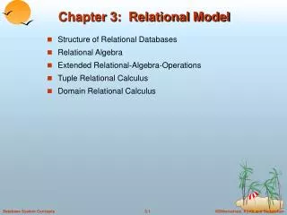
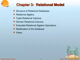
Unit 3 The Relational Model. Outline. 3.1 Introduction 3.2 Relational Data Structure 3.3 Relational Integrity Rules 3.4 Relational Algebra 3.5 Relational Calculus. 3.1 Introduction. Relational DBMS <e.g.> DB2, INGRES, SYBASE, Oracle, mySQL. Relational Data Model.

E N D
Outline • 3.1 Introduction • 3.2 Relational Data Structure • 3.3 Relational Integrity Rules • 3.4 Relational Algebra • 3.5 Relational Calculus Unit 3 The Relational Model
3.1 Introduction Unit 3 The Relational Model
Relational DBMS <e.g.> DB2, INGRES, SYBASE, Oracle, mySQL Relational Data Model Relational Model [Codd, 1970] • A way of looking at data • A prescription for • representing data: by means of tables • manipulating that representation:by select, join, ... Unit 3 The Relational Model
WORKS_IN Name Mark Dept Math_Dept Relational Model (cont.) • Concerned with three aspects of data: 1. Data structure: tables 2. Data integrity: primary key rule, foreign key rule 3. Data manipulation:(Relational Operators): • Relational Algebra (See Section 3.4) • Relational Calculus (See Section 3.5) • Basic idea: relationship expressed in data values, not in link structure. <e.g.> Entity Relationship Entity Mark Works_in Math_Dept Unit 3 The Relational Model
S# NAME STATUS CITY London Paris etc. Domains Primary key Cardinality Relation Tuples > Attributes S# S1 S2 S3 S4 S5 SNAME Smith Jones Blake Clark Adams STATUS 20 10 30 20 30 CITY London Paris Paris London Athens < Terminologies • Relation : so far corresponds to a table. • Tuple : a row of such a table. • Attribute : a column of such a table. • Cardinality : number of tuples. • Degree : number of attributes. • Primary key : an attribute or attribute combination that uniquely identify a tuple. • Domain : a pool of legal values. Degree
3.2 Relational Data Structure • Three aspects of Relational Model: • 1. Data structure: Tables • 2. Data integrity: Primary key rule, Foreign key rule • 3. Data manipulation:Relational Operators Unit 3 The Relational Model
S# SNAME STATUS CITY S1 Smith 20 London S4 Clark 20 London Relations • Definition : A relation on domains D1, D2, ..., Dn (not necessarily all distinct) consists of a heading and a body. heading body • Heading : a fixed set of attributes A1,....,An such that Aj underlying domain Dj (j=1...n) . • Body: a time-varying set of tuples. • Tuple: a set of attribute-value pairs. {A1:Vi1, A2:Vi2,..., An:Vin}, where I = 1...m or Unit 3 The Relational Model
Domain • Domain: a set of scalar values with the same type. • Scalar: the smallest semantic unit of data, atomic, nondecomposable. • Domain-Constrained Comparisons: two attributes defined on the same domain, then comparisons and hence joins, union, etc. will make sense. <e.g.> SELECT P.*, SP.* SELECT P.*, SP.*FROM P, SP FROM P, SP WHERE P.P#=SP.P# WHERE P.Weight=SP.Qty same domain different domain • A system that supports domain will prevent users from making silly mistakes. Unit 3 The Relational Model
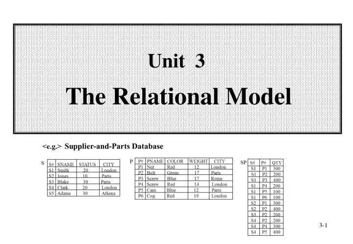
S SP S# P# QTY S1 P1 300 S1 P2 200 S1 P3 400 S1 P4 200 S1 P5 100 S1 P6 100 S2 P1 300 S2 P2 400 S3 P2 200 S4 P2 200 S4 P4 300 S4 P5 400 S# SNAME STATUS CITY S1 Smith 20 London S2 Jones 10 Paris S3 Blake 30 Paris S4 Clark 20 London S5 Adams 30 Athens P P# PNAME COLOR WEIGHT CITY P1 Nut Red 12 London P2 Bolt Green 17 Paris P3 Screw Blue 17 Rome P4 Screw Red 14 London P5 Cam Blue 12 Paris P6 Cog Red 19 London Domain (cont.) • Domain should be specified as part of the database definition. <e.g.> CREATE DOMAIN S# CHAR(5) CREATE DOMAIN NAME CHAR(20) CREATE DOMAIN STATUS SMALLINT; CREATE DOMAIN CITY CHAR(15) CREATE DOMAIN P# CHAR(6) CREATE TABLE S (S# DOMAIN (S#) Not Null SNAME DOMAIN (NAME), . . CREATE TABLE P (P# DOMAIN (P#) Not Null, PNAME DOMAIN (NAME). . . CREATE TABLE SP (S# DOMAIN (S#) Not Null, P# DOMAIN (P#) Not Null, . . <e.g.> Supplier-and-Parts Database Unit 3 The Relational Model
S S# SNAME STATUS CITY S1 Smith 20 London S2 Jones 10 Paris S3 Blake 30 Paris S4 Clark 20 London S5 Adams 30 Athens Properties of Relations • There are no duplicate tuples: since relation is a mathematical set. • Corollary : the primary key always exists. (at least the combination of all attributes of the relation has the uniqueness property.) • Tuples are unordered. • Attributes are unordered. • All attribute values are atomic. i.e. There is only one value, not a list of values at every row-and-column position within the table. i.e. Relations do not contain repeating groups. i.e. Relations are normalized. Unit 3 The Relational Model
S# S1 S2 S3 S4 PQ { (P1,300), (P2, 200), (P3, 400), (P4, 200), (P5, 100), (P6, 100) } { (P1, 300), (P2, 400) } { (P2, 200) } { (P2, 200), (P4, 300), (P5, 400) } S# S1 S1 S1 S1 S1 S1 S2 S2 S3 S4 S4 S4 P# P1 P2 P3 P4 P5 P6 P1 P2 P2 P2 P4 P5 QTY 300 200 400 200 100 100 300 400 200 200 300 400 Normalized Properties of Relations (cont.) • Normalization 1NF “fact” • degree : 2 - degree: 3 • domains: - domains: • S# = {S1, S2, S3, S4} S# = {S1, S2, S3, S4} • PQ = {<p,q> | p{P1, P2, ..., P6} P# = {P1, P2, ..., P6} • q {x| 0 x 1000}} QTY = {x| 0x 1000}} -a mathematical relation - a mathematical relation Unit 3 The Relational Model
S# S1 S2 S3 S4 PQ { (P1,300), (P2, 200), (P3, 400), (P4, 200), (P5, 100), (P6, 100) } { (P1, 300), (P2, 400) } { (P2, 200) } { (P2, 200), (P4, 300), (P5, 400) } S# S1 S1 S1 S1 S1 S1 S2 S2 S3 S4 S4 S4 P# P1 P2 P3 P4 P5 P6 P1 P2 P2 P2 P4 P5 QTY 300 200 400 200 100 100 300 400 200 200 300 400 Normalized • Reason for normalizing a relation: Simplicity!! • <e.g.> Consider two transactions T1, T2: Transaction T1 : insert ('S5', 'P6' , 500) Transaction T2 : insert ('S4', 'P6', 500) “fact” Un-normalized Normalized There are difference: • Un-normalized: two operations (one insert, one append) • Normalized: one operation (insert) Unit 3 The Relational Model
London Supplier View S P Base table Relation OP Relation Kinds of Relations • Base Relations (Real Relations): a named, atomic relation; a direct part of the database. e.g. S, P • Views (Virtual Relations): a named, derived relation; purely represented by its definition in terms of other named relations. • Snapshots: a named, derived relation with its own stored data. <e.g.> CREATE SNAPSHOT SC AS SELECT S#, CITY FROM S REFRESH EVERY DAY; • A read-only relation. • Periodically refreshed • Query Results: may or may not be named, no persistent existence within the database. • Intermediate Results: result of subquery, typically unnamed. • Temporary Relations: a named relation, automatically destroyed at some appropriate time. LS Unit 3 The Relational Model
C, Java ,PL/1 assembler machine Relational Databases • Definition: A Relational Database is a databasethat is perceived by the users as a collection oftime-varying, normalized relations. • Perceived by the users: the relational model apply at the external and conceptual levels. • Time-varying: the set of tuples changes with time. • Normalized: contains no repeating group (only contains atomic value). • The relational model represents a database system at a level of abstraction that removed from the details of the underlying machine, like high-level language. DBMS environments Relational DBMS Relational Data Model Unit 3 The Relational Model
3.3 Relational Integrity Rules Purpose: to inform the DBMS of certain constraints in the real world. Unit 3 The Relational Model
S SP S# P# QTY S1 P1 300 S1 P2 200 S1 P3 400 S1 P4 200 S1 P5 100 S1 P6 100 S2 P1 300 S2 P2 400 S3 P2 200 S4 P2 200 S4 P4 300 S4 P5 400 S# SNAME STATUS CITY S1 Smith 20 London S2 Jones 10 Paris S3 Blake 30 Paris S4 Clark 20 London S5 Adams 30 Athens Keys • Candidate keys: Let R be a relation with attributes A1, A2, ..., An. The set of attributes K (Ai, Aj, ..., Am) of R is said to be a candidate key iff it satisfies: • Uniqueness: At any time, no two tuples of R have the same value for K. • Minimum: none of Ai, Aj, ... Ak can be discarded from K without destroying the uniqueness property. <e.g.> S# in S is a candidate key. (S#, P#) in SP is a candidate key. (S#, CITY) in S is not a candidate key. • Primary key: one of the candidate keys. • Alternate keys: candidate keys which are not the primary key. <e.g.> S#, SNAME: both are candidate keys S#: primary key SNAME: alternate key. • Note: Every relation has at least one candidate key. Unit 3 The Relational Model
CK S (R1) P (R1) P# P1 P2 P3 P4 PNAME . . . . . . . . . . . S# S1 S2 S3 SNAME . . . . . . . . . reference reference SP (R2) S# S1 S1 S2 S2 S2 QTY . . . . . P# P2 P4 P1 P2 P4 Foreign keys, FK Foreign keys (p.261 of C. J . Date) • Foreign keys: Attribute FK (possibly composite) of base relation R2 is a foreign keys iff it satisfies: • 1. There exists a base relation R1 with a candidate key CK, and • 2. For all time, each value of FK is identical to the value of CK in some tuple in the current value of R1.
S SP S# P# QTY S1 P1 300 S1 P2 200 S1 P3 400 S1 P4 200 S1 P5 100 S1 P6 100 S2 P1 300 S2 P2 400 S3 P2 200 S4 P2 200 S4 P4 300 S4 P5 400 S# SNAME STATUS CITY S1 Smith 20 London S2 Jones 10 Paris S3 Blake 30 Paris S4 Clark 20 London S5 Adams 30 Athens Two Integrity Rules of Relational Model • Rule 1: Entity Integrity Rule No component of the primary key of a base relation is allowed to accept nulls. • Rule 2: Referential Integrity Rule The database must not contain any unmatched foreign key values. Note:Additional rules which is specific to the database can be given. <e.g.> QTY = { 0~1000} However, they are outside the scope of the relational model. Unit 3 The Relational Model
CK S (R1) P (R1) S# S1 S2 S3 SNAME . . . . . . . . . P# P1 P2 P4 PNAME . . . . . . . . . reference reference SP (R2) S# S1 S1 S2 S2 S2 QTY . . . . . P# P2 P4 P1 P2 P4 Foreign keys, FK Foreign Key Statement • Descriptive statements: FOREIGN KEY (foreign key) REFERENCES target NULLS [NOT] ALLOWED DELETE OF target effect UPDATE OF target-primary-key effect; effect: one of {RESTRICTED, CASCADES, NULLIFIES} <e.g.1> (p.269) CREATE TABLE SP (S# S# NOT NULL, P# P# NOT NULL, QTY QTY NOT NULL, PRIMARY KEY (S#, P#), FOREIGN KEY (S#) REFERENCE S ON DELETE CASCADE ON UPDATE CASCADE, FOREIGN KEY (P#) REFERENCE P ON DELETE CASCADE ON UPDATE CASCADE, CHECK (QTY>0 AND QTY<5001)); Unit 3 The Relational Model
S SP S# P# QTY S1 P1 300 S1 P2 200 S1 P3 400 S1 P4 200 S1 P5 100 S1 P6 100 S2 P1 300 S2 P2 400 S3 P2 200 S4 P2 200 S4 P4 300 S4 P5 400 S# SNAME STATUS CITY S1 Smith 20 London S2 Jones 10 Paris S3 Blake 30 Paris S4 Clark 20 London S5 Adams 30 Athens S SP S1 S1 S1 How to avoid against the referential Integrity Rule? • Delete rule: what should happen on an attempt to delete/update target of a foreign key reference • RESTRICTED • CASCADES • NULLIFIES <e.g.>User issues: DELETE FROM S WHERE S#='S1' System performs: Restricted: Reject! Cascades: DELETE FROM SP WHERE S#='S1' Nullifies: UPDATE SP SET S#=Null WHERE S#='S1' • FOREIGN KEY (S#) REFERENCE S • ON DELETE CASCADE • ON UPDATE CASCADE, Cascade!! Unit 3 The Relational Model
3.4 Relational Algebra • Three aspects of Relational Model: • 1. Data structure: Tables • 2. Data integrity: Primary key rule, Foreign key rule • 3. Data manipulation:Relational Operators • Relational Algebra • Relational Calculus Unit 3 The Relational Model
S SP S# P# QTY S1 P1 300 S1 P2 200 S1 P3 400 S1 P4 200 S1 P5 100 S1 P6 100 S2 P1 300 S2 P2 400 S3 P2 200 S4 P2 200 S4 P4 300 S4 P5 400 S# SNAME STATUS CITY S1 Smith 20 London S2 Jones 10 Paris S3 Blake 30 Paris S4 Clark 20 London S5 Adams 30 Athens P P# PNAME COLOR WEIGHT CITY P1 Nut Red 12 London P2 Bolt Green 17 Paris P3 Screw Blue 17 Rome P4 Screw Red 14 London P5 Cam Blue 12 Paris P6 Cog Red 19 London 3.4.1 Introduction to Relational Algebra • The relational algebra consists of a collection of eighthigh-level operators that operate on relations [defined by Codd, 1970] • Traditional set operations: • Union ( • Intersection () • Difference () • Cartesian Product / Times (x) • Special relational operations: • Restrict () or Selection • Project () • Join ( ) • Divide () <e.g.> Supplier-and-Parts Database Unit 3 The Relational Model
Relational Operators Intersection () Difference () Union ( Unit 3 The Relational Model
Divide () a a a b c x y z x y x z a Relational Operators (cont.) Restrict () Project () Product (x) a b c x y a a b b c c x y x y x y Join (Natural) • Cartesian Product / Times (x) R1 x y w R2 z x y z w a1 b1 b1 c1 a1 b1 b2 c2 a1 b1 b3 c3 a2 b1 b1 c1 . . . . . . . . . . . . a1 a2 a3 b1 b1 b2 b1 b2 b3 c1 c2 c3 a1 a2 a3 b1 b1 b2 c1 c1 c2 R1 R2 y=z R1 x R2 Unit 3 The Relational Model
+ 0 1 2 3 0 0 1 2 3 1 1 2 3 4 2 2 3 4 5 3 3 4 5 6 Relational Algebra: property of closure • The relational algebra consists of a collection of eighthigh-level operators that operate on relations. • Each operator takes relations (one or two) as operands and produce a relation as result. • the important property of closure. • nested relational expression is possible. <e.g.> R3 = (R1 R2) {{0,1,2,3},+} T1R1 join R2 R3 T1 selection Integer + 0 1 2 3 0 0 1 2 3 1 1 2 3 0 2 2 3 0 1 3 3 1 0 2 {I; +, -, *} {relations; OP1, OP2, ..., OP8} 1+2 = 3 N 5+8 = 13 N closure! objects Closure! NOT Closure! Unit 3 The Relational Model
SQL vs. Relational Operators • ASQL SELECTcontains several relational operators. <e.g.> SQL: SELECT S#, SNAME FROM S, SP WHERE S.S# = SP.S# AND CITY = 'London ‘ AND QTY > 200 SQL Language processor algebra (intermediate form) Code generator Object code • 1> S S# SP • 2> CITY ='London', QTY>200 • 3> S#,SNAME S#, SNAME (CITY='London', QTY>200 (SS# SP)) = Unit 3 The Relational Model
A B S# SNAME STATUS CITY S1 Smith 20 London S4 Clark 20 London S# SNAME STATUS CITY S1 Smith 20 London S2 Jones 10 Paris A B S# SNAME STATUS CITY S1 Smith 20 London S2 Jones 10 Paris S4 Clark 20 London 3.4.2 Traditional Set Operations • Union Compatibility: two relations are union compatible iff they have identical headings. i.e.: 1. they have same set of attribute name. 2. corresponding attributes are defined on the same domain. • objective: ensure the result is still a relation. • Union (), Intersection () and Difference () require Union Compatibility, while Cartesian Product (X) don't. Unit 3 The Relational Model
A B S# SNAME STATUS CITY S1 Smith 20 London S4 Clark 20 London S# SNAME STATUS CITY S1 Smith 20 London S2 Jones 10 Paris A B S# SNAME STATUS CITY S1 Smith 20 London S2 Jones 10 Paris S4 Clark 20 London Traditional Set Operations: UNION • A, B: two union-compatible relations. A : (X1,...,Xm) B : (X1,...,Xm) • A UNION B: • Heading: (X1,...,Xm) • Body: the set of all tuples t belonging to either A or B (or both). • Association: (A B ) C = A ( B C) • Commutative: A B = B A Unit 3 The Relational Model
A B S# SNAME STATUS CITY S1 Smith 20 London S4 Clark 20 London S# SNAME STATUS CITY S1 Smith 20 London S2 Jones 10 Paris A B S# SNAME STATUS CITY S1 Smith 20 London Traditional Set Operations: INTERSECTION • A, B: two union-compatible relations. A : (X1,...,Xm) B : (X1,...,Xm) • A INTERSECT B: • Heading: (X1,...,Xm) • Body: the set of all tuples t belonging to both A and B. • Association: (A B) C = A (B C) • Commutative: A B = B A Unit 3 The Relational Model
A B S# SNAME STATUS CITY S1 Smith 20 London S4 Clark 20 London S# SNAME STATUS CITY S1 Smith 20 London S2 Jones 10 Paris A B S# SNAME STATUS CITY S4 Clark 20 London B A S# SNAME STATUS CITY S2 Jones 20 London Traditional Set Operations: DIFFERENCE • A, B: two union-compatible relations. A : (X1,...,Xm) B : (X1,...,Xm) • A MINUS B: • Heading: (X1,...,Xm) • Body: the set of all tuples t belonging to A and not to B. • Association: No! (A B) C A ( B C ) • Commutative: No! A B B A Unit 3 The Relational Model
Traditional Set Operations: TIMES • Extended Cartesian Product (x): Given: A = { a | a= (a1,...,am)} B = { b | b= (b1,...,bn)} • Mathematical Cartesian product: A x B = { t | t=((a1,...,am),(b1,...,bn))} • Extended Cartesian Product: A x B = { t | t= (a1,...,am,b1,...,bn)} Coalescing • Product Compatibility: two relations are product-compatible iff their headings are disjoint. <e.g.1> A (S#, SNAME) B (P#, PNAME, COLOR) A and B are product compatible! math. A = {x, y} B = {y, z} A x B = {(x,y),(x,z),(y,y),(y,z)} A x B (S#, SNAME, P#, PNAME, COLOR) Unit 3 The Relational Model
Traditional Set Operations: TIMES (cont.) <e.g.2> S (S#, SNAME, STATUS, CITY) P (P#, PNAME, COLOR, WEIGHT, CITY) S and P are not product compatible! P RENAME CITY AS PCITY; S x P (S#, ..., CITY, ..., CITY) S x P (S#, ..., CITY, ..., PCITY) Unit 3 The Relational Model
B A P# P1 P2 P3 P4 P5 P6 S# S1 S2 S3 S4 S5 X Traditional Set Operations: TIMES(cont.) • A, B: two product-compatible relations. A : (X1,...,Xm), A = { a | a = (a1,...,am)} B : (Y1,...,Yn), B = { b | b = (b1,...,bn)} • A TIMES B: (A x B) • Heading: (X1,...,Xm,Y1,...,Yn) • Body: { c | c = (a1,...,am,b1,...,bn)} • Association: (A x B) x C = A x (B x C) • Commutative: A x B = B x A A X B S# S1 S1 S1 S1 S1 S1 S2 . . . S2 S3 . . . S3 S4 . . . S4 S5 . . . S5 P# P1 P2 P3 P4 P5 P6 P1 . . . P6 P1 . . . P6 P1 . . . P6 P1 . . . P6 Unit 3 The Relational Model
A X Y S S# SNAME STATUS CITY S1 Smith 20 London S2 Jones 10 Paris S3 Blake 30 Paris S4 Clark 20 London S5 Adams 30 Athens S’ S# SNAME STATUS CITY S1 Smith 20 London S4 Clark 20 London 3.4.3 Special Relational Operations • Restriction: a unary operator or monadic • Consider: A: a relation, X,Y: attributes or literal • theta-restriction (or abbreviate to just 'restriction'): A WHERE X theta Y or X theta Y (A) (By Date) (By Ullman) theta : =, <>, >, >=, <, <=, etc. • The restriction condition (X theta Y) can be extended to be any Boolean combination by including the following equivalences: C1 and C2 (A) = C1 (A) C2 (A); C1 or C2 (A) = C1 (A) C2 (A); not C (A) = A C (A) • <e.g.> S WHERE CITY='London'? or CITY='London'(S) () Unit 3 The Relational Model
COLOR Red Green Blue Blue CITY London Paris Rome Paris Special Relational Operations: Projection • Projection: a unary operator. • Consider: A : a relation X,Y,Z : attributes • A[X,Y,Z] or X,Y,Z(A) • Identity projection: A =A or (A) = A • Nullity projection: A[ ] = or (A) = • <e.g.> P[COLOR,CITY] P Unit 3 The Relational Model
Special Relational Operations: Natural Join • Natural Join: a binary operator. • Consider: A : (X1,...,Xm, Y1,...,Yn) B : (Y1,...,Yn, Z1,...,Zp) • A JOIN B (or A B): common attributes appear only once. e.g. CITY (X1,...,Xm, Y1,...,Yn, Z1,...,Zp); • Association: (A B ) C = A ( B C ) • Commutative: A B = B A • if A and B have no attribute in common, then A B = A x B Unit 3 The Relational Model
Special Relational Operations:Natural Join(cont.) • <e.g.> S JOIN P or S P S.city = P.city S.city = P.city P S CITY London S# S1 S1 S1 S2 S2 S3 S3 S4 S4 S4 SNAME Smith Smith Smith Jones Jones Blake Blake Clark Clark Clark STATUS 20 20 20 10 10 30 30 20 20 20 CITY London London London Paris Paris Paris Paris London London London P# P1 P4 P6 P2 P5 P2 P5 P1 P4 P6 PNAME Nut Screw Cog Bolt Cam Bolt Cam Nut Screw Cog COLOR Red Red Red Green Blue Green Blue Red Red Red WEIGHT 12 14 19 17 12 17 12 12 14 19 Unit 3 The Relational Model
S# S2 S2 S2 S3 S3 S3 SNAME Jones Jones Jones Blake Blake Blake STATUS 10 10 10 30 30 30 CITY Paris Paris Paris Paris Paris Paris P# P1 P4 P6 P1 P4 P6 PNAME Nut Screw Cog Nut Screw Cog COLOR Red Red Red Red Red Red WEIGHT 12 14 19 12 14 19 PCITY London London London London London London Special Relational Operations: Theta Join • A, B: product-compatible relations, A: (X1,...,Xm), B: (Y1,...,Yn) • theta : =, <>, <, >,..... • A B = X theta Y(A x B) X theta Y • If theta is '=', the join is called equijoin. <e.g.> a greater-than join SELECT S.*, P.* FROM S, P WHERE S.CITY > P.CITY CITY>PCITY(S x (P RENAME CITY AS PCITY)) Unit 3 The Relational Model
x A y S# S1 S1 S1 S1 S1 S1 S2 S2 S3 S4 S4 S4 P# P1 P2 P3 P4 P5 P6 P1 P2 P2 P2 P4 P5 B y P# P1 P2 P3 P4 P5 P6 x AB S# S1 Special Relational Operations: Division • Division: • A, B: two relations. A : (X1,...,Xm, Y1,...,Yn) B : (Y1,...,Yn) • A DIVIDEBY B (or A B): • Heading: (X1,...,Xm) • Body: all (X:x) s.t. (X:x,Y:y) in A for all (Y:y) in B • <e.g.> "Get supplier numbers for suppliers who supply all parts." Unit 3 The Relational Model
Special Relational Operations: primitive • Which of the eight relational operators are primitive? 1. UNION 2. DIFFERENCE 3. CARTESIAN PRODUCT 4. RESTRICT 5. PROJECT • How to define the non-primitive operators by those primitive operators? 1. Natural Join: S P S#,SNAME,STATUS,CITY,P#,PNAME,COLOR,WEIGHT (CITY=PCITY(S X (P RENAME CITY AS PCITY))) s.city = p.city Unit 3 The Relational Model
Special Relational Operations: primitive(cont.) 2. INTERSECT: A B = A (A B) A-(A-B) A-B A B Unit 3 The Relational Model
A[X] A S# S1 S1 S1 S1 S1 S1 S2 S2 S3 S4 S4 S4 P# P1 P2 P3 P4 P5 P6 P1 P2 P2 P2 P4 P5 S# S1 S2 S3 S4 B P# P1 P2 P3 P4 P5 P6 . A [X] B - A (A [X] B - A) [X] S# S2 S2 S2 S2 S3 S3 S3 S3 S3 S4 S4 S4 P# P3 P4 P5 P6 P1 P3 P4 P5 P6 P1 P3 P6 S# S2 S3 S4 Special Relational Operations: primitive(cont.)) 3. DIVIDE: A B = A[X] - (A[X] B - A)[X] A [X] B S# S1 . . . S1 S2 . . . S2 S3 . . . S3 S4 . . . S4 P# P1 . . . P6 P1 . . . P6 P1 . . . P6 P1 . . . P6 A[X] - (A [X] B - A) [X] . S# S1 Unit 3 The Relational Model
3.4.4 BNF Grammars for Relational Operator 1. expression ::= monadic-expression | dyadic-expression 2. monadic-expression ::= renaming | restriction | projection 3. renaming ::= term RENAME attribute AS attribute 4. term ::= relation | (expression ) 5. restriction ::= term WHERE condition 6. Projection ::= attribute | term [attribute-commalist] 7. dyadic-expression ::= projection dyadic-operation expression 8. dyadic-operation ::= UNION | INTERSECT | MINUS | TIMES | JOIN | DIVIDEBY e.g. 1. S [S#, SNAME] e.g.2 S Join P term term term attri-commalist dyadic exp Unit 3 The Relational Model
exp 1 dyadic-expression 7 7 7 projection dyadic-operation expression 6 8 1 JOIN term monadic-expression 2 4 projection relation S 6 term 4 relation P BNF Grammars for Relational Operator (cont.) e.g. S JOIN P Unit 3 The Relational Model
Relational Algebra V.S. Database Language: • Example : Get supplier name for suppliers who supply part P2. • SQL: SELECT S.SNAME FROM S, SP WHERE S.S# = SP.S# AND SP.P# = 'P2' • Relational algebra: (( S JOIN SP) WHERE P# = 'P2') [SNAME] SNAME (P#='P2' (S SP)) or Unit 3 The Relational Model
What is the Algebra for? (1) Allow writing of expressions which serve as a high-level (SQL) and symbolic representation of the users intend. (2) Symbolic transformation rules are possible. A convenient basis for optimization! e.g. (( S JOIN SP ) WHERE P#='P2')[SNAME] = (S JOIN ( SP WHERE P#='P2')) [SNAME] Back to p.3-61 Unit 3 The Relational Model
3.5 Relational Calculus • Three aspects of Relational Model: • 1. Data structure: Tables • 2. Data integrity: Primary key rule, Foreign key rule • 3. Data manipulation:Relational Operators • Relational Algebra • Relational Calculus Unit 3 The Relational Model
New P# CITY SP S 3.5.1 Introduction to Relational Calculus • A notation for expressing the definition of some new relations in terms of some given relations. <e.g.> SP.P#, S.CITY WHERE SP.S# = S.S# definition predicate • Based on first order predicate calculus (a branch of mathematical logic). • Originated by Kuhn for database language (1967). • Proposed by Codd for relational database (1972) • ALPHA: a language based on calculus, never be implemented. • QUEL: query language of INGRES, influenced by ALPHA. • Two forms : • Tuple calculus: by Codd.. • Domain calculus: by Lacroix and Pirotte. Unit 3 The Relational Model
S S# SNAME STATUS CITY S1 Smith 20 London S2 Jones 10 Paris S3 Blake 30 Paris S4 Clark 20 London S5 Adams 30 Athens Tuple Calculus • BNF Grammar: <e.g.> "Get supplier number for suppliers in Paris with status > 20" Tuple calculus expression: SX.S# WHERE SX.CITY='Paris' and SX.STATUS>20 tuple attribute WFF (Well-Formed Formula) variable Unit 3 The Relational Model