Applications of Remote Sensing: The Cryosphere (Snow & Ice)

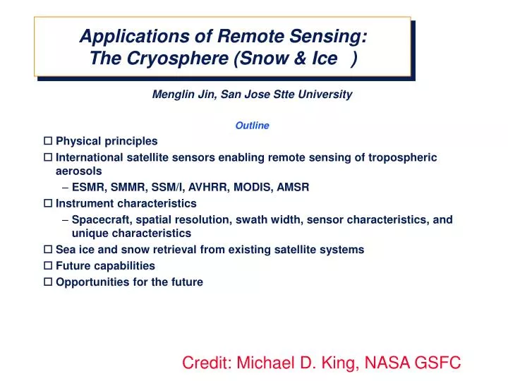
1. Applications of Remote Sensing:The Cryosphere (Snow & Ice) Menglin Jin, San Jose Stte University Outline • Physical principles • International satellite sensors enabling remote sensing of tropospheric aerosols • ESMR, SMMR, SSM/I, AVHRR, MODIS, AMSR • Instrument characteristics • Spacecraft, spatial resolution, swath width, sensor characteristics, and unique characteristics • Sea ice and snow retrieval from existing satellite systems • Future capabilities • Opportunities for the future Credit: Michael D. King, NASA GSFC

2. Sea Ice of Different Forms and Perspectives • Sparsely distributed ice floes as viewed from a ship in the Bering Sea Photograph courtesy of Claire Parkinson

3. Sea Ice of Different Forms and Perspectives • Expansive ice field, as viewed from an aircraft in the central Arctic Photograph courtesy of Claire Parkinson

4. Sea Ice of Different Forms and Perspectives • Close-up of newly formed ice in the Bering Sea Photograph courtesy of Claire Parkinson

5. Sea Ice of Different Forms and Perspectives • Ice floes separated by a lead, as viewed from an aircraft over the central Arctic Photograph courtesy of Claire Parkinson

6. Sea Ice of Different Forms and Perspectives • Thin sheets of ice, as viewed from an aircraft Photograph courtesy of Koni Steffen

7. Sea Ice of Different Forms and Perspectives • Several-months-old ice bearing the weight of a helicopter, as viewed from ground level in the Bering Sea Photograph courtesy of Claire Parkinson

8. Remote Sensing of Sea Ice from Passive Microwave Radiometers • Nimbus 5 • Electrically Scanning Microwave Radiometer (ESMR) • December 1972-1976 • single channel (19 GHz = 1.55 cm) conically scanning microwave radiometer • Nimbus 7 • Scanning Multichannel Microwave Radiometer (SMMR) • October 1978-August 1987 • 10 channel (five frequency and dual polarization) conically scanning microwave radiometer • Defense Meteorological Satellite Program (DMSP) • Special Sensor Microwave Imager (SSM/I) • June 1987-present • 7 channel (three frequencies with both vertical and horizontal polarization + 1 frequency with horizontal polarization only)

9. Advanced Microwave Scanning Radiometer (AMSR-E) • NASA, Aqua • launches July 2001 • 705 km polar orbits, ascending (1:30 p.m.) • Sensor Characteristics • 12 channel microwave radiometer with 6 frequencies from 6.9 to 89.0 GHz with both vertical and horizontal polarization • conical scan mirror with 55° incident angle at Earth’s surface • Spatial resolutions: • 6 x 4 km (89.0 GHz) • 75 x 43 km (6.9 GHz) • External cold load reflector and a warm load for calibration • 1 K Tb accuracy

10. Microwave Scattering of Snow Cover • Thicker snow results in lower microwave brightness temperatures From Parkinson, C. L., 1997: Earth from Above

11. Satellite Detection of Sea Ice • Higher rate of microwave emission from sea ice than from open water • Emissivities indicated are for wavelength of 1.55 cm (19 GHz) From Parkinson, C. L., 1997: Earth from Above

12. Spectra of Polar Oceanic Surfaces over the SMMR Wavelengths 250 FY Ice V FY Ice H 200 MY Ice V MY Ice H Open Ocean V 150 Brightness Temperature (K) 100 Open Ocean H 50 0 0.0 0.5 1.0 1.5 2.0 2.5 3.0 3.5 4.0 4.5 5.0 Wavelength (cm)

13. Brightness Temperature of Polar Regions from Nimbus 5 ESMR March 8-10, 1974 September 16-18, 1974 <132.5 K 140 K 160 K 180 K 200 K 220 K 240 K 260 K ≥ 281.5 K Tb (19 GHz) Parkinson ( 1997)

14. Monthly Average Sea Ice Concentrations from Nimbus 7 SMMR 100% 80% 60% 40% 20% ≤12% March 1986 September 1986 From Parkinson, C. L., 1997: Earth from Above

15. Monthly Average Sea Ice Concentrations from Nimbus 7 SMMR March 1986 September 1986 100% 80% 60% 40% 20% ≤12% From Parkinson, C. L., 1997: Earth from Above

16. Monthly Average Sea Ice Concentrations from SSM/I February 1999 September 1999 100% 80% 60% 40% 20% ≤12%

17. Location Maps for North and South Polar Regions North Polar Region South Polar Region From Parkinson, C. L., 1997: Earth from Above

18. Decreases in Arctic Sea Ice Coverage as Observed from Satellite Observations November 1978 - December 1996 C. L. Parkinson, D. J. Cavalieri, P. Gloersen, H. J. Zwally, and J. C. Comiso, 1999: J. Geophys. Res.

19. Monthly Arctic Sea Ice Extent Deviations November 1978 - December 1996 –34300 ± 3700 km2/year C. L. Parkinson, D. J. Cavalieri, P. Gloersen, H. J. Zwally, and J. C. Comiso, 1999: J. Geophys. Res.

20. Trends in Arctic Sea Ice Coverage Yearly and Seasonal Ice Extent Trends Yearly –2.8%/decade Winter –2.2%/decade Spring –3.1%/decade Summer –4.5%/decade Autumn –1.9%/decade • Data Sources • For November 1978 – August 1987, the Scanning Multichannel Microwave Radiometer (SMMR) on NASA’s Nimbus 7 satellite • Since mid-August 1987, the Special Sensor Microwave Imagers (SSM/Is) on satellites of the Defense Meteorological Satellite Program • 37,000 km2/year decrease of sea ice area over a 19.4 year period observed from satellite • 19,000 km2/year decrease in sea ice area over a 46 year period based on Geophysical Fluid Dynamics Laboratory (GFDL) model C. L. Parkinson, D. J. Cavalieri, P. Gloersen, H. J. Zwally, and J. C. Comiso, 1999: J. Geophys. Res.

21. Observed Northern Hemisphere Sea Ice Decreases Placed in a Climate Context Probability that an observed sea-ice-extent trend results from natural climate variability, based on a 5000-year control run of the GFDL General Circulation Model (GCM) • Open Circle • Observed 1953-1998 trend, updated from Chapman and Walsh (1993) • Open Square • Observed 1978-1998 trend, updated from Parkinson et al. (1999)

22. Sea Ice Trends • Probability that observed trends result from natural climate variability • 1953 – 1998 trend < 0.1 % • 1978 – 1998 trend < 2 % • Demonstrates how scientists have attempted to take the satellite data record and put it into context of man’s impact on climate Vinnikov, Robock, Stouffer, Walsh, Parkinson, Cavalieri, Mitchell, Garrett, and Zakharov, published in the December 3, 1999 issue of Science

23. Brightness Temperature of Polar Regions from SSM/I March 14, 1997 19 GHz Vertical Polarization 37 GHz Vertical Polarization <132.5 K 140 K 160 K 180 K 200 K 220 K 240 K 260 K ≥ 281.5 K

24. Brightness Temperature of Polar Regions from SSM/I March 14, 1997 85 GHz Vertical Polarization <132.5 K 140 K 160 K 180 K 200 K 220 K 240 K 260 K ≥ 281.5 K

25. Brightness Temperature Scatter Diagram for Odden Region and Greenland Sea Early Ice Maximum Extent of Bulge November 21, 1996 January 18, 1997 260 A Thick ice (consolidated region) A 240 D Brightness Temperature (V19) D 220 Odden Study Area (pancakes or nilas) 200 180 O O 180 200 220 240 260 180 200 220 240 260 Brightness Temperature (V37) Brightness Temperature (V37)

26. Brightness Temperature Scatter Diagram for Odden Region and Greenland Sea Maximum Extent of Tongue Ice Melt & Formation of Ice Island March 14, 1997 April 14, 1997 260 240 Brightness Temperature (V19) 220 200 180 180 200 220 240 260 180 200 220 240 260 Brightness Temperature (V37) Brightness Temperature (V37)

27. Brightness Temperature of Polar Regions from SSM/I SSM/I AVHRR February 26, 1987

28. Brightness Temperature of Polar Regions from SSM/I SSM/I AVHRR March 15, 1987

29. Snow Cover in the Northern Andes • Pucahirca, Peru • October 1991 • Latitude of 9°S • Foreground altitude is 5325 m Photograph courtesy of Lonnie Thompson

30. Remote Sensing of Snow Cover & Thickness from Passive Microwave Radiometers • Nimbus 7/SMMR • Uses two horizontally polarized microwave frequencies (18 and 37 GHz) • snow scatters less at the lower frequency (longer wavelength) • the thicker the snow the greater the difference in brightness temperature between 18 and 37 GHz Dz = 1.59[Tb(18 GHz) – Tb(37 GHz)] where z = snow thickness in cm • restricted to ice-free land with snow thickness 5 ≤ z ≤ 70 cm

31. Monthly Average Snow Thickness from Nimbus 7 SMMR 70 cm 55 cm 40 cm 25 cm 10 cm ≤4 cm March 1986 February 1986 From Parkinson, C. L., 1997: Earth from Above

32. Monthly Average Snow Thickness from Nimbus 7 SMMR 70 cm 55 cm 40 cm 25 cm 10 cm ≤4 cm April 1986 May 1986 From Parkinson, C. L., 1997: Earth from Above

33. Location Map for North Polar Region From Parkinson, C. L., 1997: Earth from Above

34. Monthly Average Snow Thickness from Nimbus 7 SMMR 70 cm 55 cm 40 cm 25 cm 10 cm ≤4 cm February 1979 February 1981 From Parkinson, C. L., 1997: Earth from Above

35. Remote Sensing of Snow Cover from Shortwave Infrared Radiometers • NOAA/AVHRR-3 • Uses reflectance at 1.6 µm where snow and ice absorb solar radiation much greater than water or vegetation • Advantage • high spatial resolution (4 km GAC, 1.1 km LAC) • Disadvantage • affected by cloud cover • observations possible only at night • difficult to detect snow in deep forests • Terra/MODIS • Uses reflectance at 1.6 µm • Higher spatial resolution of AVHRR (global at 1 km) • Makes use of better cloud mask for distinguishing clouds from snow and land surfaces (and shadows)

36. MODIS Snow Cover Compared to Historical Snow Record March 5-12, 2000 (1966-present) March Average February Average Cloud