Download
1 / 55
560 likes | 746 Vues
Quantum transport and its classical limit. Piet Brouwer Laboratory of Atomic and Solid State Physics Cornell University. Lecture 1 Capri spring school on Transport in Nanostructures, March 25-31, 2007. Quantum Transport.

E N D
Quantum transport and its classical limit Piet Brouwer Laboratory of Atomic and Solid State Physics Cornell University Lecture 1 Capri spring school on Transport in Nanostructures, March 25-31, 2007
Quantum Transport About the manifestations of quantum mechanics on the electrical transport properties of conductors sample These lectures: signatures of quantum interference • Quantum effects not covered here: • Interaction effects • Shot noise • Mesoscopic superconductivity
Quantum Transport These lectures: signatures of quantum interference What to expect? G1+2 (e2/h) G(e2/h) dG B (mT) G1=G2=2e2/h B (10-4T) B R1+2=R1+R2 Magnetofingerprint Nonlocality Figures adapted from: Mailly and Sanquer (1991) Webb, Washburn, Umbach, and Laibowitz (1985) Marcus (2005)
Landauer-Buettiker formalism Ideal leads sample y W x N: number of propagating transverse modes or “channels” N depends on energy e, width W an: electrons moving towards sample bn: electrons moving away from sample Note: |an|2 and |bn|2 determine flux in each channel, not density
Scattering Matrix: Definition • More than one lead: • Nj is number of channels in lead j • Use amplitudes anj, bnj for incoming, • outgoing electrons, n = 1, …, Nj. sample Linear relationship between anj, bnj: S: “scattering matrix” • |Smj;nk|2 describes what fraction of the flux of electrons entering in lead k, • channel n, leaves sample through lead j, channel m. • Probability that an electron entering in lead k, channel n, leaves sample • through lead j, channel m is|Smj;nk|2 vnk/vmj.
Scattering matrix: Properties Linear relationship between anj, bnj: sample S: “scattering matrix” • Current conservation: S is unitary • Time-reversal symmetry: If y is a solution of the Schroedinger equation at magnetic field B, theny* is a solution at magnetic field –B.
Landauer-Buettiker formalism Reservoirs Each lead j is connected to an electron reservoir at temperature T and chemical potential mj. sample mj, T Distribution function for electrons originating from reservoir j is f(e-mj).
Landauer-Buettiker formalism Current in leads sample Ij,in Ij,out mj, T In one dimension: = (nnkh)-1 Buettiker (1985)
Landauer-Buettiker formalism Linear response mj = m – eVj sample Expand to first order in Vj: Ij,in Ij,out mj, T Zero temperature
Conductance coefficients sample • Current conservation • and gauge invariance Ij mj=m-eVj • Time-reversal Note: only if B=0 or if there are only two leads. Otherwise and in general.
Multiterminal measurements In four-terminal measurement, one measures a combination of the 16 coefficients Gjk. Different ways to perform the measurement correspond to different combinations of the Gjk, so they give different results! V I V I I V Benoit, Washburn, Umbach, Laibowitz, Webb (1986)
Landauer formula: spin • Without spin-dependent scattering: Factor two for spin • degeneracy • With spin-dependent scattering: Use separate sets of • channels for each spin direction. Dimension of scattering • matrix is doubled. Conductance measured in units of 2e2/h: “Dimensionless conductance”.
Two-terminal geometry r’ t r, r’: “reflection matrices” t, t’: “transmission matrices” r t’ in e e f(e) f(e) eV out e e e (meV) f(e) Anthore, Pierre, Pothier, Devoret (2003) |t’|2 |r|2 |t|2 |r’|2
Quantum transport Landauer formula r’ t r t’ sample What is the “sample”? • Point contact • Quantum dot • Disordered metal wire • Metal ring • Molecule • Graphene sheet
Example: adiabatic point contact N(x) Nmin g 10 x 8 6 4 2 Vgate (V) 0 -2.0 -1.8 -1.6 -1.4 -1.2 -1.0 Van Wees et al. (1988)
Quantum interference a In general: dg small, random sign b tnm,a , tnm,b : amplitude for transmission along paths a, b
Quantum interference • Three prototypical examples: • Disordered wire • Disordered quantum dot • Ballistic quantum dot
Scattering matrix and Green function Recall: retarded Green function is solution of In one dimension: Green function in channel basis: ek = e and v = h-1dek/dk r in lead j; r’ in lead k Substitute 1d form of Green function If j = k:
Quantum transport and its classical limit Piet Brouwer Laboratory of Atomic and Solid State Physics Cornell University Lecture 2 Capri spring school on Transport in Nanostructures, March 25-31, 2007
Characteristic time scales lF l L t tD tH h/eF terg Elastic mean free time Inverse level spacing: relevant for closed samples Ballistic quantum dot: t ~ terg ~ L/vF, l ~ L Diffusive conductor: terg ~ L2/D
Characteristic conductances Conductances of the contacts: g1, g2 Conductance of sample without contacts:gsample if g >> 1 • ‘Bulk measurement’: g1,2 >> gsample • Quantum dot:g1,2 << gsample g dominated by sample g dominated by contacts general relationships:
Assumptions and restrictions Always: lF << l. Well-defined momentum between scattering events Diagrammatic perturbation theory: g >> 1. This implies tD << tH Only ‘nonperturbative’ methods can describe the regime g ~ 1 or, equivalently, times up to tH. Examples are certain field theories, random matrix theory.
G Quantum interference corrections Weak localization Small negative correction to the ensemble-averaged conductance at zero magnetic field Conductance fluctuations Reproducible fluctuations of the sample-specific conductance as a function of magnetic field or Fermi energy B G B Anderson, Abrahams, Ramakrishnan (1979) Gorkov, Larkin, Khmelnitskii (1979) Altshuler (1985) Lee and Stone (1985)
Weak localization (1) Nonzero (negative) ensemble average dg at zero magnetic field g dg B a = + b + permutations ‘Hikami box’ ‘Cooperon’ Interfering trajectories propagating in opposite directions
Weak localization (2) Nonzero (negative) ensemble average dg at zero magnetic field g dg B Sign of effect follows directly from quantum correction to reflection. a b Trajectories propagating at the same angle in the leads contribute to the same element of the reflection matrix r. Such trajectories can interfere.
Weak localization (3) Disordered wire: (no derivation here) G(e2/h) Disordered quantum dot: B (10-4T) N1 channels N2 channels (derivation later) Mailly and Sanquer (1991) a b F
Weak localization (4) dg G(e2/h) B (10-4T) a Magnetic field suppresses WL. 10-3 DR/R b 0 H(kOe) F -10-3 Chentsov (1948)
Weak localization (5) a b F Typical dwell time for transmitted electrons: terg Typical area enclosed in that time: sample area A. WL suppressed at flux F ~ hc/e through sample. Typical area enclosed in time terg: sample area A. Typical area enclosed in timetD: A(tD/terg)1/2. WL suppressed at F ~ (hc/e)(terg/tD)1/2 << hc/e.
Weak localization (6) b In a ring, all trajectories enclose multiples of the same area. If F is a multiple of hc/2e, all phase differences are multiples of 2p : dg oscillates with period hc/2e. a F ‘hc/2e Aharonov-Bohm effect’ Altshuler, Aronov, Spivak (1981) Note: phases picked up by individual trajectories are multiples of p, not 2p! Sharvin and Sharvin (1981)
Conductance fluctuations (1) Fluctuations of dg with applied magnetic field dg Umbach, Washburn, Laibowitz, Webb (1984) a b a b “diffuson” interfering trajectories in the same direction b’ a’ a’ b’ a a “cooperon” interfering trajectories in the opposite direction b b a’ a’ b’ b’
Conductance fluctuations (2) Fluctuations of dg with applied magnetic field dg Disordered wire: G(e2/h) Disordered quantum dot: B (mT) N1 channels N2 channels Jalabert, Pichard, Beenakker (1994) Baranger and Mello (1994) Marcus (2005)
Conductance fluctuations (3) dg b F a In a ring: sample-specific conductance g is periodic funtion of F with period hc/e. ‘hc/e Aharonov-Bohm effect’ Webb, Washburn, Umbach, and Laibowitz (1985)
Random Matrix Theory Quantum dot Ideal contacts: every electron that reaches the contact is transmitted. For ideal contacts: all elements of S have random phase. N1 channels N2 channels Ansatz: S is as random as possible, with constraints of unitarity and time-reversal symmetry, “Dyson’s circular ensemble” Dimension of S is N1+N2. Assign channels m=1, …, N1 to lead 1, channels m=N1+1, …, N1+N2 to lead 2 Bluemel and Smilansky (1988)
RMT: Without time-reversal symmetry Quantum dot Ansatz: S is as random as possible, with constraint of unitarity • Probability to find certain S does not change if • We permute rows or columns • We multiply a row or column by eif N1 channels N2 channels Average conductance: No interference correction to average conductance
RMT: with time-reversal symmetry Quantum dot Additional constraint: • Probability to find certain S does not change if • We permute rows and columns, • We multiply a row and columns by eif, • while keeping S symmetric N1 channels N2 channels Average conductance: Interference correction to average conductance
RMT: with time-reversal symmetry Quantum dot Weak localization correction is difference with classical conductance N1 channels N2 channels For N1, N2 >> 1: Jalabert, Pichard, Beenakker (1994) Baranger and Mello (1994) Same as diagrammatic perturbation theory
RMT: conductance fluctuations Quantum dot Without time-reversal symmetry: With time-reversal symmetry: N1 channels N2 channels Jalabert, Pichard, Beenakker (1994) Baranger and Mello (1994) Same as diagrammatic perturbation theory There exist extensions of RMT to deal with contacts that contain tunnel barriers, magnetic-field dependence, etc.
Quantum transport and its classical limit Piet Brouwer Laboratory of Atomic and Solid State Physics Cornell University Lecture 3 Capri spring school on Transport in Nanostructures, March 25-31, 2007
Ballistic quantum dots • Past lectures: • Qualitative microscopic picture of interference • corrections in disordered conductors; • Quantitative calculations can be done using • diagrammatic perturbation theory • Quantitative non-microscopic theory of • interference corrections in quantum dots (RMT). This lecture: Microscopic theory of interference corrections in ballistic quantum dots Assumptions and restrictions: lF << l, g >> 1 Method: semiclassics, quantum properties are obtained from the classical dynamics
Semiclassical Green function Relation between transmission matrix and Green function Semiclassical Green function (two dimensions) a: classical trajectory connection r’ and r S: classical action ofa ma: Maslov index Aa: stability amplitude a q’ r r r’ ’
Comparison to exact Green function Semiclassical Green function (two dimensions) Exact Green function (two dimensions) Asymptotic behavior for k|r-r’| >> 1 equals semiclassical Green function
Semiclassical scattering matrix Insert semiclassical Green function and Fourier transform to y, y’. This replaces y, y’ by the conjugate momenta py, py’ and fixes these to Result: Jalabert, Baranger, Stone (1990) Legendre transformed action q a y
Semiclassical scattering matrix Transmission matrix transverse momenta of a fixed at Legendre transformed action q a Stability amplitude y Reflection matrix
Diagonal approximation Reflection probability a b Dominant contribution from terms a = b. probability to return to contact 1
Enhanced diagonal reflection Reflection probability b=a a If m=n: also contribution if b = a time-reversed of a: Without magnetic field: a and a have equal actions, hence Factor-two enhancement of diagonal reflection Doron, Smilansky, Frenkel (1991) Lewenkopf, Weidenmueller (1991)
diagonal approximation: limitations We found b=a a One expects a corresponding reduction of the transmission. Where is it? The diagonal approximation gives Note: Time-reversed of transmitting trajectories contribute to t’, not t. No interference! Compare to RMT: captured by diagonal approximation missed by diagonal approximation
Lesson from disordered metals a Weak localization correction to reflection: Do not need Hikami box. b Weak localization correction to transmission: Need Hikami box. a = + b + permutations ‘Hikami box’
Ballistic Hikami box? In a quantum dot with smooth boundaries: Wavepackets follow classical trajectories.
Ballistic Hikami box? But… quantum interference corrections dg and varg exist in ballistic quantum dots! Marcus group
Ballistic Hikami box? l: Lyapunov exponent Initial uncertainty is magnified by chaotic boundary scattering. Time until initial uncertainty ~lF has reached dot size ~L: Aleiner and Larkin (1996) Richter and Sieber (2002) Interference corrections in ballistic quantum dot same as in disordered quantum dot if tE << tD L=lF exp(l t) t = “Ehrenfest time”